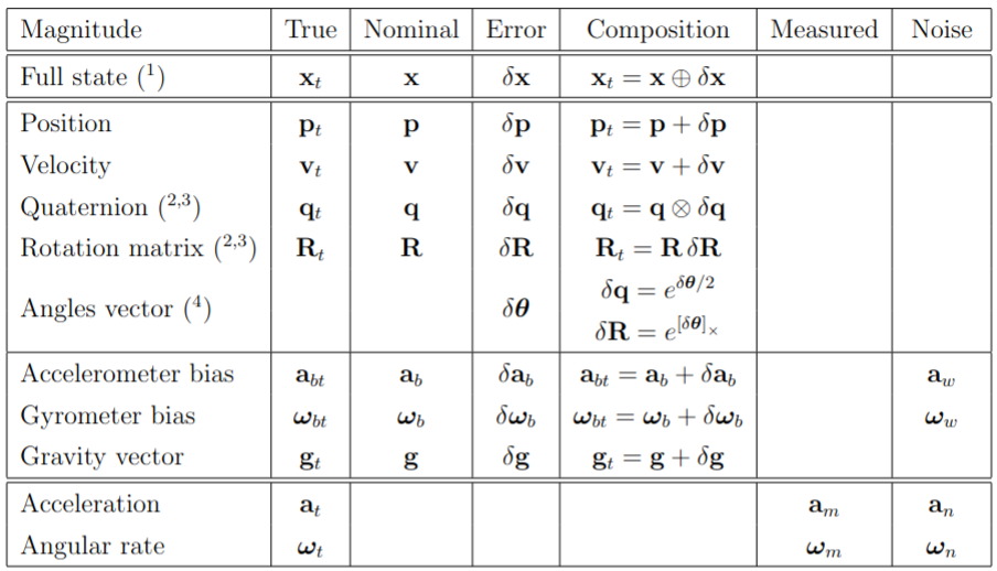
Error state Kalman filter in brief ¶ In error-state filter formulations, we speak of true-, nominal- and error-state values, the true-state being expressed as a suitable composition (linear sum, quaternion product or matrix product) of the nominal- and the error- states. The idea is to consider the nominal-state as large-signal (integrable in non-linear fashion) and the error-state as small signal (thus linearly integrable and suitable for linear-Gaussian filtering).
The error-state filter can be explained as follows. On one side, high-frequency IMU data u m u_{m} u m x x x w w w δ x δx δ x
The simplified ESKF goes like this:
Use IMU to propagate mean simply by ignoring noise
Error state equations give you state transition and noise jacobians. These are only needed for covariance propagation. Mean of error state is zero.
Update step updates the covariance using measurement jacobians and the mean error state which is injected into the mean as the next estimate.
Solas Prediction ¶ Note: Sola uses Hamilton convention. Please check the assumptions in Solas paper.
For continuos system of equations:
True state Kinematics ¶ The true acceleration a t \mathbf{a}_t a t ω t \omega_t ω t a m \mathbf{a}_m a m ω m \omega_m ω m
a m = R t ⊤ ( a t − g t ) + a b t + a n \mathbf{a}_m = \mathbf{R}_t^\top (\mathbf{a}_t - \mathbf{g}_t) + \mathbf{a}_{bt} + \mathbf{a}_n a m = R t ⊤ ( a t − g t ) + a b t + a n ω m = ω t + ω b t + ω n \omega_m = \omega_t + \omega_{bt} + \omega_n ω m = ω t + ω b t + ω n with R t ≜ R { q t } \mathbf{R}_t \triangleq \mathbf{R}\{\mathbf{q}_t\} R t ≜ R { q t }
a t = R t ( a m − a b t − a n ) + g t \mathbf{a}_t = \mathbf{R}_t(\mathbf{a}_m - \mathbf{a}_{bt} - \mathbf{a}_n) + \mathbf{g}_t a t = R t ( a m − a b t − a n ) + g t ω t = ω m − ω b t − ω n \omega_t = \omega_m - \omega_{bt} - \omega_n ω t = ω m − ω b t − ω n Substituting above yields the kinematic system
p ˙ t = v t \dot{\mathbf{p}}_t = \mathbf{v}_t p ˙ t = v t v ˙ t = R t ( a m − a b t − a n ) + g t \dot{\mathbf{v}}_t = \mathbf{R}_t(\mathbf{a}_m - \mathbf{a}_{bt} - \mathbf{a}_n) + \mathbf{g}_t v ˙ t = R t ( a m − a b t − a n ) + g t q ˙ t = 1 2 q t ⊗ ( ω m − ω b t − ω n ) \dot{\mathbf{q}}_t = \frac{1}{2} \mathbf{q}_t \otimes (\omega_m - \omega_{bt} - \omega_n) q ˙ t = 2 1 q t ⊗ ( ω m − ω b t − ω n ) a ˙ b t = a w \dot{\mathbf{a}}_{bt} = \mathbf{a}_w a ˙ b t = a w ω ˙ b t = ω w \dot{\omega}_{bt} = \omega_w ω ˙ b t = ω w g ˙ t = 0 \dot{\mathbf{g}}_t = 0 g ˙ t = 0 which we may name x ˙ t = f t ( x t , u , w ) \dot{\mathbf{x}}_t = f_t(\mathbf{x}_t, \mathbf{u}, \mathbf{w}) x ˙ t = f t ( x t , u , w ) x t \mathbf{x}_t x t u m \mathbf{u}_m u m w \mathbf{w} w
x t = [ p t v t q t a b t ω b t g t ] u = [ a m − a n ω m − ω n ] w = [ a w ω w ] \mathbf{x}_t = \begin{bmatrix} \mathbf{p}_t \\ \mathbf{v}_t \\ \mathbf{q}_t \\ \mathbf{a}_{bt} \\ \omega_{bt} \\ \mathbf{g}_t \end{bmatrix} \quad \mathbf{u} = \begin{bmatrix} \mathbf{a}_m - \mathbf{a}_n \\ \omega_m - \omega_n \end{bmatrix} \quad \mathbf{w} = \begin{bmatrix} \mathbf{a}_w \\ \omega_w \end{bmatrix} x t = ⎣ ⎡ p t v t q t a b t ω b t g t ⎦ ⎤ u = [ a m − a n ω m − ω n ] w = [ a w ω w ] Nominal state Kinematics ¶ The nominal-state kinematics corresponds to the modeled system without noises or perturbations,
p ˙ = v \dot{\mathbf{p}} = \mathbf{v} p ˙ = v v ˙ = R ( a m − a b ) + g \dot{\mathbf{v}} = \mathbf{R}(\mathbf{a}_m - \mathbf{a}_b) + \mathbf{g} v ˙ = R ( a m − a b ) + g q ˙ = 1 2 q ⊗ ( ω m − ω b ) \dot{\mathbf{q}} = \frac{1}{2} \mathbf{q} \otimes (\omega_m - \omega_b) q ˙ = 2 1 q ⊗ ( ω m − ω b ) a ˙ b = 0 \dot{\mathbf{a}}_b = 0 a ˙ b = 0 ω ˙ b = 0 \dot{\omega}_b = 0 ω ˙ b = 0 g ˙ = 0. \dot{\mathbf{g}} = 0. g ˙ = 0. Error-state kinematics ¶ The goal is to determine the linearized dynamics of the error-state. For each state equation, we write its composition, linearizing wherever needed, solving for the error state and simplifying all second-order infinitesimals.
δ p ˙ = δ v \dot{\delta \mathbf{p}} = \delta \mathbf{v} δ p ˙ = δ v δ v ˙ = − R ⌊ a m − a b ⌋ × δ θ − R δ a b + δ g − R a n \dot{\delta \mathbf{v}} = -\mathbf{R} \lfloor \mathbf{a}_m - \mathbf{a}_b \rfloor_\times \delta \theta - \mathbf{R} \delta \mathbf{a}_b + \delta \mathbf{g} - \mathbf{R} \mathbf{a}_n δ v ˙ = − R ⌊ a m − a b ⌋ × δ θ − R δ a b + δ g − R a n δ θ ˙ = − ⌊ ω m − ω b ⌋ × δ θ − δ ω b − ω n \dot{\delta \theta} = -\lfloor \omega_m - \omega_b \rfloor_\times \delta \theta - \delta \omega_b - \omega_n δ θ ˙ = − ⌊ ω m − ω b ⌋ × δ θ − δ ω b − ω n δ a ˙ b = a w \dot{\delta \mathbf{a}}_b = \mathbf{a}_w δ a ˙ b = a w δ ω ˙ b = ω w \dot{\delta \omega}_b = \omega_w δ ω ˙ b = ω w δ g ˙ = 0. \dot{\delta \mathbf{g}} = 0. δ g ˙ = 0. Now we move to discrete case:
True state Kinematics ¶ The above true state kinematics for the continuous case can be converted to true state by converting those equations into difference equations. It should be straightforward.
Nominal state Kinematics ¶ We can write the differences equations of the nominal-state as
p ← p + v Δ t + 1 2 ( R ( a m − a b ) + g ) Δ t 2 \mathbf{p} \leftarrow \mathbf{p} + \mathbf{v} \Delta t + \frac{1}{2}(\mathbf{R}(\mathbf{a}_m - \mathbf{a}_b) + \mathbf{g}) \Delta t^2 p ← p + v Δ t + 2 1 ( R ( a m − a b ) + g ) Δ t 2 v ← v + ( R ( a m − a b ) + g ) Δ t \mathbf{v} \leftarrow \mathbf{v} + (\mathbf{R}(\mathbf{a}_m - \mathbf{a}_b) + \mathbf{g}) \Delta t v ← v + ( R ( a m − a b ) + g ) Δ t q ← q ⊗ q { ( ω m − ω b ) Δ t } \mathbf{q} \leftarrow \mathbf{q} \otimes \mathbf{q} \{ (\omega_m - \omega_b) \Delta t \} q ← q ⊗ q {( ω m − ω b ) Δ t } a b ← a b \mathbf{a}_b \leftarrow \mathbf{a}_b a b ← a b ω b ← ω b \omega_b \leftarrow \omega_b ω b ← ω b g ← g , \mathbf{g} \leftarrow \mathbf{g}, g ← g , where x ← f ( x , ∙ ) x \leftarrow f(x, \bullet) x ← f ( x , ∙ ) x k + 1 = f ( x k , ∙ k ) x_{k+1} = f(x_k, \bullet_k) x k + 1 = f ( x k , ∙ k ) R ≜ R { q } \mathbf{R} \triangleq \mathbf{R}\{\mathbf{q}\} R ≜ R { q } q \mathbf{q} q q { v } \mathbf{q}\{v\} q { v } v v v
We can also use more precise integration. Check RK4 methods.
Error-state kinematics ¶ The deterministic part is integrated normally, and the integration of the stochastic part results in random impulses, thus,
δ p ← δ p + δ v Δ t \delta \mathbf{p} \leftarrow \delta \mathbf{p} + \delta \mathbf{v} \Delta t δ p ← δ p + δ v Δ t δ v ← δ v + ( − R ⌊ a m − a b ⌋ × δ θ − R δ a b + δ g ) Δ t + v i \delta \mathbf{v} \leftarrow \delta \mathbf{v} + (-\mathbf{R} \lfloor \mathbf{a}_m - \mathbf{a}_b \rfloor_\times \delta \theta - \mathbf{R} \delta \mathbf{a}_b + \delta \mathbf{g}) \Delta t + \mathbf{v}_{\mathbf{i}} δ v ← δ v + ( − R ⌊ a m − a b ⌋ × δ θ − R δ a b + δ g ) Δ t + v i δ θ ← R ⊤ { ( ω m − ω b ) Δ t } δ θ − δ ω b Δ t + θ i \delta \theta \leftarrow \mathbf{R}^\top \{ (\omega_m - \omega_b) \Delta t \} \delta \theta - \delta \omega_b \Delta t + \theta_{\mathbf{i}} δ θ ← R ⊤ {( ω m − ω b ) Δ t } δ θ − δ ω b Δ t + θ i δ a b ← δ a b + a i \delta \mathbf{a}_b \leftarrow \delta \mathbf{a}_b + \mathbf{a}_{\mathbf{i}} δ a b ← δ a b + a i δ ω b ← δ ω b + ω i \delta \omega_b \leftarrow \delta \omega_b + \omega_{\mathbf{i}} δ ω b ← δ ω b + ω i δ g ← δ g . \delta \mathbf{g} \leftarrow \delta \mathbf{g}. δ g ← δ g . Here, v i \mathbf{v}_{\mathbf{i}} v i θ i \theta_{\mathbf{i}} θ i a i \mathbf{a}_{\mathbf{i}} a i ω i \omega_{\mathbf{i}} ω i a n , ω n , a w \mathbf{a}_n, \omega_n, \mathbf{a}_w a n , ω n , a w ω w \omega_w ω w Δ t \Delta t Δ t
V i = σ a n 2 Δ t 2 I [ m 2 / s 2 ] \mathbf{V}_{\mathbf{i}} = \sigma_{\mathbf{a}_n}^2 \Delta t^2 \mathbf{I} \quad [m^2/s^2] V i = σ a n 2 Δ t 2 I [ m 2 / s 2 ] Θ i = σ ω n 2 Δ t 2 I [ r a d 2 ] \Theta_{\mathbf{i}} = \sigma_{\omega_n}^2 \Delta t^2 \mathbf{I} \quad [rad^2] Θ i = σ ω n 2 Δ t 2 I [ r a d 2 ] A i = σ a w 2 Δ t I [ m 2 / s 4 ] \mathbf{A}_{\mathbf{i}} = \sigma_{\mathbf{a}_w}^2 \Delta t \mathbf{I} \quad [m^2/s^4] A i = σ a w 2 Δ t I [ m 2 / s 4 ] Ω i = σ ω w 2 Δ t I [ r a d 2 / s 2 ] \Omega_{\mathbf{i}} = \sigma_{\omega_w}^2 \Delta t \mathbf{I} \quad [rad^2/s^2] Ω i = σ ω w 2 Δ t I [ r a d 2 / s 2 ] where σ a n [ m / s 2 ] \sigma_{\mathbf{a}_n} [m/s^2] σ a n [ m / s 2 ] σ ω n [ r a d / s ] \sigma_{\omega_n} [rad/s] σ ω n [ r a d / s ] σ a w [ m / s 2 s ] \sigma_{\mathbf{a}_w} [m/s^2\sqrt{s}] σ a w [ m / s 2 s ] σ ω w [ r a d / s s ] \sigma_{\omega_w} [rad/s\sqrt{s}] σ ω w [ r a d / s s ]
Error-state Jacobian and perturbation matrices ¶ The Jacobians are obtained by simple inspection of the error-state differences equations in the previous section.
To write these equations in compact form, we consider the nominal state vector x \mathbf{x} x δ x \delta \mathbf{x} δ x u m \mathbf{u}_m u m i \mathbf{i} i
x = [ p v q a b ω b g ] , δ x = [ δ p δ v δ θ δ a b δ ω b δ g ] , u m = [ a m ω m ] , i = [ v i θ i a i ω i ] \mathbf{x} = \begin{bmatrix} \mathbf{p} \\ \mathbf{v} \\ \mathbf{q} \\ \mathbf{a}_b \\ \omega_b \\ \mathbf{g} \end{bmatrix} , \quad \delta \mathbf{x} = \begin{bmatrix} \delta \mathbf{p} \\ \delta \mathbf{v} \\ \delta \theta \\ \delta \mathbf{a}_b \\ \delta \omega_b \\ \delta \mathbf{g} \end{bmatrix} , \quad \mathbf{u}_m = \begin{bmatrix} \mathbf{a}_m \\ \omega_m \end{bmatrix} , \quad \mathbf{i} = \begin{bmatrix} \mathbf{v}_{\mathbf{i}} \\ \theta_{\mathbf{i}} \\ \mathbf{a}_{\mathbf{i}} \\ \omega_{\mathbf{i}} \end{bmatrix} x = ⎣ ⎡ p v q a b ω b g ⎦ ⎤ , δ x = ⎣ ⎡ δ p δ v δ θ δ a b δ ω b δ g ⎦ ⎤ , u m = [ a m ω m ] , i = ⎣ ⎡ v i θ i a i ω i ⎦ ⎤ The error-state system is now
δ x ← f ( x , δ x , u m , i ) = F x ( x , u m ) ⋅ δ x + F i ⋅ i , \delta \mathbf{x} \leftarrow f(\mathbf{x}, \delta \mathbf{x}, \mathbf{u}_m, \mathbf{i}) = \mathbf{F}_{\mathbf{x}}(\mathbf{x}, \mathbf{u}_m) \cdot \delta \mathbf{x} + \mathbf{F}_{\mathbf{i}} \cdot \mathbf{i}, δ x ← f ( x , δ x , u m , i ) = F x ( x , u m ) ⋅ δ x + F i ⋅ i , The ESKF prediction equations are written:
δ x ^ ← F x ( x , u m ) ⋅ δ x ^ \hat{\delta \mathbf{x}} \leftarrow \mathbf{F}_{\mathbf{x}}(\mathbf{x}, \mathbf{u}_m) \cdot \hat{\delta \mathbf{x}} δ x ^ ← F x ( x , u m ) ⋅ δ x ^ P ← F x P F x ⊤ + F i Q i F i ⊤ , \mathbf{P} \leftarrow \mathbf{F}_{\mathbf{x}} \mathbf{P} \mathbf{F}_{\mathbf{x}}^\top + \mathbf{F}_{\mathbf{i}} \mathbf{Q}_{\mathbf{i}} \mathbf{F}_{\mathbf{i}}^\top , P ← F x P F x ⊤ + F i Q i F i ⊤ , where δ x ∼ N { δ x ^ , P } 25 \delta \mathbf{x} \sim \mathcal{N}\{\hat{\delta \mathbf{x}}, \mathbf{P}\}^{25} δ x ∼ N { δ x ^ , P } 25 F x \mathbf{F}_{\mathbf{x}} F x F i \mathbf{F}_{\mathbf{i}} F i f ( ) f() f ( ) Q i \mathbf{Q}_{\mathbf{i}} Q i
The expressions of the Jacobian and covariances matrices above are detailed below. All state-related values appearing herein are extracted directly from the nominal state.
F x = ∂ f ∂ δ x ∣ x , u m = [ I I Δ t 0 0 0 0 0 I − R ⌊ a m − a b ⌋ × Δ t − R Δ t 0 I Δ t 0 0 R ⊤ { ( ω m − ω b ) Δ t } 0 − I Δ t 0 0 0 0 I 0 0 0 0 0 0 I 0 0 0 0 0 0 I ] \mathbf{F}_{\mathbf{x}} = \left. \frac{\partial f}{\partial \delta \mathbf{x}} \right|_{\mathbf{x}, \mathbf{u}_m} = \begin{bmatrix}
\mathbf{I} & \mathbf{I} \Delta t & 0 & 0 & 0 & 0 \\
0 & \mathbf{I} & -\mathbf{R} \lfloor \mathbf{a}_m - \mathbf{a}_b \rfloor_\times \Delta t & -\mathbf{R} \Delta t & 0 & \mathbf{I} \Delta t \\
0 & 0 & \mathbf{R}^\top \{ (\omega_m - \omega_b) \Delta t \} & 0 & -\mathbf{I} \Delta t & 0 \\
0 & 0 & 0 & \mathbf{I} & 0 & 0 \\
0 & 0 & 0 & 0 & \mathbf{I} & 0 \\
0 & 0 & 0 & 0 & 0 & \mathbf{I}
\end{bmatrix} F x = ∂ δ x ∂ f ∣ ∣ x , u m = ⎣ ⎡ I 0 0 0 0 0 I Δ t I 0 0 0 0 0 − R ⌊ a m − a b ⌋ × Δ t R ⊤ {( ω m − ω b ) Δ t } 0 0 0 0 − R Δ t 0 I 0 0 0 0 − I Δ t 0 I 0 0 I Δ t 0 0 0 I ⎦ ⎤ F i = ∂ f ∂ i ∣ x , u m = [ 0 0 0 0 I 0 0 0 0 I 0 0 0 0 I 0 0 0 0 I 0 0 0 0 ] , Q i = [ V i 0 0 0 0 Θ i 0 0 0 0 A i 0 0 0 0 Ω i ] . \mathbf{F}_{\mathbf{i}} = \left. \frac{\partial f}{\partial \mathbf{i}} \right|_{\mathbf{x}, \mathbf{u}_m} = \begin{bmatrix}
0 & 0 & 0 & 0 \\
\mathbf{I} & 0 & 0 & 0 \\
0 & \mathbf{I} & 0 & 0 \\
0 & 0 & \mathbf{I} & 0 \\
0 & 0 & 0 & \mathbf{I} \\
0 & 0 & 0 & 0
\end{bmatrix} \quad , \quad \mathbf{Q}_{\mathbf{i}} = \begin{bmatrix}
\mathbf{V}_{\mathbf{i}} & 0 & 0 & 0 \\
0 & \Theta_{\mathbf{i}} & 0 & 0 \\
0 & 0 & \mathbf{A}_{\mathbf{i}} & 0 \\
0 & 0 & 0 & \Omega_{\mathbf{i}}
\end{bmatrix} . F i = ∂ i ∂ f ∣ ∣ x , u m = ⎣ ⎡ 0 I 0 0 0 0 0 0 I 0 0 0 0 0 0 I 0 0 0 0 0 0 I 0 ⎦ ⎤ , Q i = ⎣ ⎡ V i 0 0 0 0 Θ i 0 0 0 0 A i 0 0 0 0 Ω i ⎦ ⎤ . Openvins Prediction ¶ Note: Openvins uses JPL convention. Please check the papers for assumptions.
Referenes:
As before we start with the continuos case.
True state kinematics ¶ Openvins state is of the form:
x I ( t ) = [ G I q ˉ ( t ) G p I ( t ) G v I ( t ) b g ( t ) b a ( t ) ] \mathbf{x}_I(t) = \begin{bmatrix} {^I_G\bar{q}}(t) \\ {^G\mathbf{p}_I}(t) \\ {^G\mathbf{v}_I}(t) \\ \mathbf{b}_g(t) \\ \mathbf{b}_a(t) \end{bmatrix} x I ( t ) = ⎣ ⎡ G I q ˉ ( t ) G p I ( t ) G v I ( t ) b g ( t ) b a ( t ) ⎦ ⎤ The IMU state evolves over time as follows:
G I q ˉ ˙ ( t ) = 1 2 [ − ⌊ I ω ( t ) × ⌋ I ω ( t ) − I ω ( t ) ⊤ 0 ] G I t q ˉ {^I_G\dot{\bar{q}}}(t) = \frac{1}{2} \begin{bmatrix} -\lfloor ^I\omega(t) \times \rfloor & ^I\omega(t) \\ -^I\omega(t)^\top & 0 \end{bmatrix} {^{I_t}_G\bar{q}} G I q ˉ ˙ ( t ) = 2 1 [ − ⌊ I ω ( t ) × ⌋ − I ω ( t ) ⊤ I ω ( t ) 0 ] G I t q ˉ ≜ 1 2 Ω ( I ω ( t ) ) G I t q ˉ \triangleq \frac{1}{2} \Omega(^I\omega(t)) {^{I_t}_G\bar{q}} ≜ 2 1 Ω ( I ω ( t )) G I t q ˉ G p ˙ I ( t ) = G v I ( t ) {^G\dot{\mathbf{p}}_I}(t) = {^G\mathbf{v}_I}(t) G p ˙ I ( t ) = G v I ( t ) G v ˙ I ( t ) = G I t R ⊤ I a ( t ) {^G\dot{\mathbf{v}}_I}(t) = {^{I_t}_G\mathbf{R}}^\top {^I\mathbf{a}}(t) G v ˙ I ( t ) = G I t R ⊤ I a ( t ) b ˙ g ( t ) = n w g ( t ) \dot{\mathbf{b}}_{\mathbf{g}}(t) = \mathbf{n}_{wg}(t) b ˙ g ( t ) = n w g ( t ) b ˙ a ( t ) = n w a ( t ) \dot{\mathbf{b}}_{\mathbf{a}}(t) = \mathbf{n}_{wa}(t) b ˙ a ( t ) = n w a ( t ) where we have modeled the gyroscope and accelerometer biases as random walk and thus their time derivatives are white Gaussian. Note that the above kinematics have been defined in terms of the true acceleration and angular velocities which can be computed as a function of the sensor measurements and state.
Continuous-time Inertial Integration ¶ Given the continuous-time I ω ( t ) ^I\omega(t) I ω ( t ) I a ( t ) ^I\mathbf{a}(t) I a ( t ) t ∈ [ t k , t k + 1 ] t \in [t_k, t_{k+1}] t ∈ [ t k , t k + 1 ] I ω ^ ( t ) ^I\hat{\omega}(t) I ω ^ ( t ) I a ^ ( t ) ^I\hat{\mathbf{a}}(t) I a ^ ( t )
G I k + 1 R = exp ( − ∫ t k t k + 1 I ω ( t τ ) d τ ) G I k R {^{I_{k+1}}_G\mathbf{R}} = \exp \left( -\int_{t_k}^{t_{k+1}} {}^I\omega(t_\tau) \, d\tau \right) {^{I_k}_G\mathbf{R}} G I k + 1 R = exp ( − ∫ t k t k + 1 I ω ( t τ ) d τ ) G I k R ≜ Δ R k G I k R = I k I k + 1 R G I k R \triangleq \Delta\mathbf{R}_k {^{I_k}_G\mathbf{R}} = {^{I_{k+1}}_{I_k}\mathbf{R}} {^{I_k}_G\mathbf{R}} ≜ Δ R k G I k R = I k I k + 1 R G I k R G p I k + 1 = G p I k + G v I k Δ t k + G I k R ⊤ ∫ t k t k + 1 ∫ t k s I τ I k R I a ( t τ ) d τ d s − 1 2 G g Δ t k 2 {^G\mathbf{p}_{I_{k+1}}} = {^G\mathbf{p}_{I_k}} + {^G\mathbf{v}_{I_k}} \Delta t_k + {^{I_k}_G\mathbf{R}}^\top \int_{t_k}^{t_{k+1}} \int_{t_k}^{s} {^{I_k}_{I_\tau}\mathbf{R}} {}^I\mathbf{a}(t_\tau) \, d\tau ds - \frac{1}{2} {}^G\mathbf{g} \Delta t_k^2 G p I k + 1 = G p I k + G v I k Δ t k + G I k R ⊤ ∫ t k t k + 1 ∫ t k s I τ I k R I a ( t τ ) d τ d s − 2 1 G g Δ t k 2 ≜ G p I k + G v I k Δ t k + G I k R ⊤ Δ p k − 1 2 G g Δ t k 2 \triangleq {^G\mathbf{p}_{I_k}} + {^G\mathbf{v}_{I_k}} \Delta t_k + {^{I_k}_G\mathbf{R}}^\top \Delta \mathbf{p}_k - \frac{1}{2} {}^G\mathbf{g} \Delta t_k^2 ≜ G p I k + G v I k Δ t k + G I k R ⊤ Δ p k − 2 1 G g Δ t k 2 G v I k + 1 = G v I k + G I k R ⊤ ∫ t k t k + 1 I τ I k R I a ( t τ ) d τ − G g Δ t k {^G\mathbf{v}_{I_{k+1}}} = {^G\mathbf{v}_{I_k}} + {^{I_k}_G\mathbf{R}}^\top \int_{t_k}^{t_{k+1}} {^{I_k}_{I_\tau}\mathbf{R}} {}^I\mathbf{a}(t_\tau) \, d\tau - {}^G\mathbf{g} \Delta t_k G v I k + 1 = G v I k + G I k R ⊤ ∫ t k t k + 1 I τ I k R I a ( t τ ) d τ − G g Δ t k ≜ G v I k + G I k R ⊤ Δ v k − G g Δ t k \triangleq {^G\mathbf{v}_{I_k}} + {^{I_k}_G\mathbf{R}}^\top \Delta \mathbf{v}_k - {}^G\mathbf{g} \Delta t_k ≜ G v I k + G I k R ⊤ Δ v k − G g Δ t k b g k + 1 = b g k + ∫ t k t k + 1 n w g ( t τ ) d τ \mathbf{b}_{g_{k+1}} = \mathbf{b}_{g_k} + \int_{t_k}^{t_{k+1}} \mathbf{n}_{wg}(t_\tau) \, d\tau b g k + 1 = b g k + ∫ t k t k + 1 n w g ( t τ ) d τ b a k + 1 = b a k + ∫ t k t k + 1 n w a ( t τ ) d τ \mathbf{b}_{a_{k+1}} = \mathbf{b}_{a_k} + \int_{t_k}^{t_{k+1}} \mathbf{n}_{wa}(t_\tau) \, d\tau b a k + 1 = b a k + ∫ t k t k + 1 n w a ( t τ ) d τ where Δ t k = t k + 1 − t k \Delta t_k = t_{k+1} - t_k Δ t k = t k + 1 − t k I τ I k R = exp ( ∫ t k t τ I ω ( t u ) d u ) {^{I_k}_{I_\tau}\mathbf{R}} = \exp(\int_{t_k}^{t_\tau} {}^I\omega(t_u) \, du) I τ I k R = exp ( ∫ t k t τ I ω ( t u ) d u ) exp ( ⋅ ) \exp(\cdot) exp ( ⋅ ) S O ( 3 ) SO(3) SO ( 3 ) G v I k = G v I ( t k ) {^G\mathbf{v}_{I_k}} = {^G\mathbf{v}_I}(t_k) G v I k = G v I ( t k ) n w g \mathbf{n}_{wg} n w g n w a \mathbf{n}_{wa} n w a
Δ R k ≜ I k I k + 1 R = exp ( − ∫ t k t k + 1 I ω ( t τ ) d τ ) \Delta \mathbf{R}_k \triangleq {^{I_{k+1}}_{I_k}\mathbf{R}} = \exp \left( -\int_{t_k}^{t_{k+1}} {}^I\omega(t_\tau) \, d\tau \right) Δ R k ≜ I k I k + 1 R = exp ( − ∫ t k t k + 1 I ω ( t τ ) d τ ) Δ p k ≜ ∫ t k t k + 1 ∫ t k s I τ I k R I a ( t τ ) d τ d s \Delta \mathbf{p}_k \triangleq \int_{t_k}^{t_{k+1}} \int_{t_k}^{s} {^{I_k}_{I_\tau}\mathbf{R}} {}^I\mathbf{a}(t_\tau) \, d\tau ds Δ p k ≜ ∫ t k t k + 1 ∫ t k s I τ I k R I a ( t τ ) d τ d s Δ v k ≜ ∫ t k t k + 1 I τ I k R I a ( t τ ) d τ \Delta \mathbf{v}_k \triangleq \int_{t_k}^{t_{k+1}} {^{I_k}_{I_\tau}\mathbf{R}} {}^I\mathbf{a}(t_\tau) \, d\tau Δ v k ≜ ∫ t k t k + 1 I τ I k R I a ( t τ ) d τ Openvins Discrete Propagation ¶ True state ¶ Assumptions:
Simple IMU model
Hold initial measuement constant over the period including R which in pratice changes since angular velocity is constant over the interval
We model the measurements as discrete-time over the integration period. To do this, the measurements can be assumed to be constant during the sampling period. We employ this assumption and approximate that the measurement at time t k t_k t k t k + 1 t_{k+1} t k + 1 ω m ( t k ) = ω m , k \omega_m(t_k) = \omega_{m,k} ω m ( t k ) = ω m , k a m ( t k ) = a m , k \mathbf{a}_m(t_k) = \mathbf{a}_{m,k} a m ( t k ) = a m , k t ∈ [ t k , t k + 1 ] t \in [t_k, t_{k+1}] t ∈ [ t k , t k + 1 ] k k k t k t_k t k
G p I k + 1 = G p I k + G v I k Δ t k − 1 2 G g Δ t k 2 + 1 2 G I k R ⊤ ( a m , k − b a , k − n a , k ) Δ t k 2 {^G\mathbf{p}_{I_{k+1}}} = {^G\mathbf{p}_{I_k}} + {^G\mathbf{v}_{I_k}} \Delta t_k - \frac{1}{2} {^G\mathbf{g}} \Delta t_k^2 + \frac{1}{2} {^{I_k}_G \mathbf{R}}^\top (\mathbf{a}_{m,k} - \mathbf{b}_{a,k} - \mathbf{n}_{a,k}) \Delta t_k^2 G p I k + 1 = G p I k + G v I k Δ t k − 2 1 G g Δ t k 2 + 2 1 G I k R ⊤ ( a m , k − b a , k − n a , k ) Δ t k 2 G v k + 1 = G v I k − G g Δ t k + G I k R ⊤ ( a m , k − b a , k − n a , k ) Δ t k {^G\mathbf{v}_{k+1}} = {^G\mathbf{v}_{I_k}} - {^G\mathbf{g}} \Delta t_k + {^{I_k}_G \mathbf{R}}^\top (\mathbf{a}_{m,k} - \mathbf{b}_{a,k} - \mathbf{n}_{a,k}) \Delta t_k G v k + 1 = G v I k − G g Δ t k + G I k R ⊤ ( a m , k − b a , k − n a , k ) Δ t k G I k + 1 q ˉ ^ = exp ( 1 2 Ω ( ω m , k − b g , k − n g , k ) Δ t k ) G I k q ˉ ^ {^{I_{k+1}}_G \hat{\bar{q}}} = \exp \left( \frac{1}{2} \Omega(\omega_{m,k} - \mathbf{b}_{g,k} - \mathbf{n}_{g,k}) \Delta t_k \right) {^{I_k}_G \hat{\bar{q}}} G I k + 1 q ˉ ^ = exp ( 2 1 Ω ( ω m , k − b g , k − n g , k ) Δ t k ) G I k q ˉ ^ b g , k + 1 = b g , k + n w g , k \mathbf{b}_{g,k+1} = \mathbf{b}_{g,k} + \mathbf{n}_{wg,k} b g , k + 1 = b g , k + n w g , k b a , k + 1 = b a , k + n w a , k \mathbf{b}_{a,k+1} = \mathbf{b}_{a,k} + \mathbf{n}_{wa,k} b a , k + 1 = b a , k + n w a , k where Δ t k = t k + 1 − t k \Delta t_k = t_{k+1} - t_k Δ t k = t k + 1 − t k
Note that the noises used here are the discrete ones which need to be converted from their continuous-time versions. In particular, when the covariance matrix of the continuous-time measurement noises is given by Q c \mathbf{Q}_c Q c n c = [ n g c n a c n w g c n w a c ] ⊤ \mathbf{n}_c = [\mathbf{n}_{g_c} \mathbf{n}_{a_c} \mathbf{n}_{wg_c} \mathbf{n}_{wa_c}]^\top n c = [ n g c n a c n w g c n w a c ] ⊤ Q d \mathbf{Q}_d Q d
σ g = 1 Δ t σ w c \sigma_g = \frac{1}{\sqrt{\Delta t}} \sigma_{w_c} σ g = Δ t 1 σ w c σ ω g = Δ t σ ω g c \sigma_{\omega g} = \sqrt{\Delta t} \sigma_{\omega g_c} σ ω g = Δ t σ ω g c Q m e a s = [ 1 Δ t σ g c 2 I 3 0 3 0 3 1 Δ t σ a c 2 I 3 ] \mathbf{Q}_{meas} = \begin{bmatrix} \frac{1}{\Delta t} \sigma_{g_c}^2 \mathbf{I}_3 & \mathbf{0}_3 \\ \mathbf{0}_3 & \frac{1}{\Delta t} \sigma_{a_c}^2 \mathbf{I}_3 \end{bmatrix} Q m e a s = [ Δ t 1 σ g c 2 I 3 0 3 0 3 Δ t 1 σ a c 2 I 3 ] Q b i a s = [ Δ t σ w g c 2 I 3 0 3 0 3 Δ t σ w a c 2 I 3 ] \mathbf{Q}_{bias} = \begin{bmatrix} \Delta t \sigma_{wg_c}^2 \mathbf{I}_3 & \mathbf{0}_3 \\ \mathbf{0}_3 & \Delta t \sigma_{wa_c}^2 \mathbf{I}_3 \end{bmatrix} Q bia s = [ Δ t σ w g c 2 I 3 0 3 0 3 Δ t σ w a c 2 I 3 ] where n = [ n g n a n w g n w a ] ⊤ \mathbf{n} = [\mathbf{n}_g \mathbf{n}_a \mathbf{n}_{wg} \mathbf{n}_{wa}]^\top n = [ n g n a n w g n w a ] ⊤
Q d = [ Q m e a s 0 3 0 3 Q b i a s ] \mathbf{Q}_d = \begin{bmatrix} \mathbf{Q}_{meas} & \mathbf{0}_3 \\ \mathbf{0}_3 & \mathbf{Q}_{bias} \end{bmatrix} Q d = [ Q m e a s 0 3 0 3 Q bia s ] Nominal and Error state kinematics ¶ For the error propagation the method of computing Jacobians is to “perturb” each variable in the system and see how the old error “perturbation” relates to the new error state:
G I k + 1 R = I k I k + 1 R G I k R {^{I_{k+1}}_G \mathbf{R}} = {^{I_{k+1}}_{I_k}\mathbf{R}} {^{I_k}_G\mathbf{R}} G I k + 1 R = I k I k + 1 R G I k R ( I 3 − ⌊ G I k + 1 θ ~ × ⌋ ) G I k + 1 R ^ ≈ exp ( − I k ω ^ Δ t k − I k ω ~ Δ t k ) ( I 3 − ⌊ G I k θ ~ × ⌋ ) (\mathbf{I}_3 - \lfloor {^{I_{k+1}}_G\tilde{\theta}} \times \rfloor) {^{I_{k+1}}_G\hat{\mathbf{R}}} \approx \exp(-{^{I_k}\hat{\omega}} \Delta t_k - {^{I_k}\tilde{\omega}} \Delta t_k) (\mathbf{I}_3 - \lfloor {^{I_k}_G\tilde{\theta}} \times \rfloor) ( I 3 − ⌊ G I k + 1 θ ~ × ⌋) G I k + 1 R ^ ≈ exp ( − I k ω ^ Δ t k − I k ω ~ Δ t k ) ( I 3 − ⌊ G I k θ ~ × ⌋) = I k I k + 1 R ^ ( I 3 − ⌊ J r ( − I k ω ^ Δ t k ) ω ~ k Δ t k × ⌋ ) ( I 3 − ⌊ G I k θ ~ × ⌋ ) = {^{I_{k+1}}_{I_k}\hat{\mathbf{R}}} (\mathbf{I}_3 - \lfloor \mathbf{J}_r(-{^{I_k}\hat{\omega}} \Delta t_k) \tilde{\omega}_k \Delta t_k \times \rfloor) (\mathbf{I}_3 - \lfloor {^{I_k}_G\tilde{\theta}} \times \rfloor) = I k I k + 1 R ^ ( I 3 − ⌊ J r ( − I k ω ^ Δ t k ) ω ~ k Δ t k × ⌋) ( I 3 − ⌊ G I k θ ~ × ⌋) G p I k + 1 = G p I k + G v I k Δ t k − 1 2 G g Δ t k 2 + 1 2 G I k R ⊤ a k Δ t k 2 {^G\mathbf{p}_{I_{k+1}}} = {^G\mathbf{p}_{I_k}} + {^G\mathbf{v}_{I_k}} \Delta t_k - \frac{1}{2} {^G\mathbf{g}} \Delta t_k^2 + \frac{1}{2} {^{I_k}_G\mathbf{R}}^\top \mathbf{a}_k \Delta t_k^2 G p I k + 1 = G p I k + G v I k Δ t k − 2 1 G g Δ t k 2 + 2 1 G I k R ⊤ a k Δ t k 2 G p ^ I k + 1 + G p ~ I k + 1 ≈ G p ^ I k + G p ~ I k + G v ^ I k Δ t k + G v ~ I k Δ t k − 1 2 G g Δ t k 2 + 1 2 G I k R ^ ⊤ ( I 3 + ⌊ G I k θ ~ × ⌋ ) ( a ^ k + a ~ k ) Δ t k 2 {^G\hat{\mathbf{p}}_{I_{k+1}}} + {^G\tilde{\mathbf{p}}_{I_{k+1}}} \approx {^G\hat{\mathbf{p}}_{I_k}} + {^G\tilde{\mathbf{p}}_{I_k}} + {^G\hat{\mathbf{v}}_{I_k}} \Delta t_k + {^G\tilde{\mathbf{v}}_{I_k}} \Delta t_k - \frac{1}{2} {^G\mathbf{g}} \Delta t_k^2 + \frac{1}{2} {^{I_k}_G\hat{\mathbf{R}}^\top} (\mathbf{I}_3 + \lfloor {^{I_k}_G\tilde{\theta}} \times \rfloor)(\hat{\mathbf{a}}_{k} + \tilde{\mathbf{a}}_{k})\Delta t_k^2 G p ^ I k + 1 + G p ~ I k + 1 ≈ G p ^ I k + G p ~ I k + G v ^ I k Δ t k + G v ~ I k Δ t k − 2 1 G g Δ t k 2 + 2 1 G I k R ^ ⊤ ( I 3 + ⌊ G I k θ ~ × ⌋) ( a ^ k + a ~ k ) Δ t k 2 G v k + 1 = G v I k − G g Δ t k + G I k R ⊤ a k Δ t k {^G\mathbf{v}_{k+1}} = {^G\mathbf{v}_{I_k}} - {^G\mathbf{g}} \Delta t_k + {^{I_k}_G\mathbf{R}}^\top \mathbf{a}_k \Delta t_k G v k + 1 = G v I k − G g Δ t k + G I k R ⊤ a k Δ t k G v ^ k + 1 + G v ~ k + 1 ≈ G v ^ I k + G v ~ I k − G g Δ t k + G I k R ^ ⊤ ( I 3 + ⌊ G I k θ ~ × ⌋ ) ( a ^ k + a ~ k ) Δ t k {^G\hat{\mathbf{v}}_{k+1}} + {^G\tilde{\mathbf{v}}_{k+1}} \approx {^G\hat{\mathbf{v}}_{I_k}} + {^G\tilde{\mathbf{v}}_{I_k}} - {^G\mathbf{g}} \Delta t_k + {^{I_k}_G\hat{\mathbf{R}}^\top} (\mathbf{I}_3 + \lfloor {^{I_k}_G\tilde{\theta}} \times \rfloor)(\hat{\mathbf{a}}_{k} + \tilde{\mathbf{a}}_{k})\Delta t_k G v ^ k + 1 + G v ~ k + 1 ≈ G v ^ I k + G v ~ I k − G g Δ t k + G I k R ^ ⊤ ( I 3 + ⌊ G I k θ ~ × ⌋) ( a ^ k + a ~ k ) Δ t k b g , k + 1 = b g , k + n w g \mathbf{b}_{g,k+1} = \mathbf{b}_{g,k} + \mathbf{n}_{wg} b g , k + 1 = b g , k + n w g b ^ g , k + 1 + b ~ g , k + 1 = b ^ g , k + b ~ g , k + n w g \hat{\mathbf{b}}_{g,k+1} + \tilde{\mathbf{b}}_{g,k+1} = \hat{\mathbf{b}}_{g,k} + \tilde{\mathbf{b}}_{g,k} + \mathbf{n}_{wg} b ^ g , k + 1 + b ~ g , k + 1 = b ^ g , k + b ~ g , k + n w g b a , k + 1 = b a , k + n w a \mathbf{b}_{a,k+1} = \mathbf{b}_{a,k} + \mathbf{n}_{wa} b a , k + 1 = b a , k + n w a b ^ a , k + 1 + b ~ a , k + 1 = b ^ a , k + b ~ a , k + n w a \hat{\mathbf{b}}_{a,k+1} + \tilde{\mathbf{b}}_{a,k+1} = \hat{\mathbf{b}}_{a,k} + \tilde{\mathbf{b}}_{a,k} + \mathbf{n}_{wa} b ^ a , k + 1 + b ~ a , k + 1 = b ^ a , k + b ~ a , k + n w a where ω ~ = ω − ω ^ = − ( b ~ g + n g ) \tilde{\omega} = \omega - \hat{\omega} = -(\tilde{\mathbf{b}}_g + \mathbf{n}_g) ω ~ = ω − ω ^ = − ( b ~ g + n g ) J r ( θ ) \mathbf{J}_r(\theta) J r ( θ ) S O ( 3 ) SO(3) SO ( 3 ) I k I k + 1 θ ^ = − I k ω ^ Δ t k {^{I_{k+1}}_{I_k}\hat{\theta}} = -{^{I_k}\hat{\omega}} \Delta t_k I k I k + 1 θ ^ = − I k ω ^ Δ t k a ~ = a − a ^ = − ( b ~ a + n a ) \tilde{\mathbf{a}} = \mathbf{a} - \hat{\mathbf{a}} = -(\tilde{\mathbf{b}}_a + \mathbf{n}_a) a ~ = a − a ^ = − ( b ~ a + n a )
G p ~ I k + 1 = G p ~ I k + G v ~ I k Δ t k − 1 2 G I k R ^ ⊤ ⌊ a ^ k Δ t k 2 × ⌋ G I k θ ~ − 1 2 G I k R ^ ⊤ Δ t k 2 ( b ~ a , k + n a , k ) {^G\tilde{\mathbf{p}}_{I_{k+1}}} = {^G\tilde{\mathbf{p}}_{I_k}} + {^G\tilde{\mathbf{v}}_{I_k}} \Delta t_k - \frac{1}{2} {^{I_k}_G\hat{\mathbf{R}}^\top} \lfloor \hat{\mathbf{a}}_k \Delta t_k^2 \times \rfloor {^{I_k}_G\tilde{\theta}} - \frac{1}{2} {^{I_k}_G\hat{\mathbf{R}}^\top} \Delta t_k^2 (\tilde{\mathbf{b}}_{a,k} + \mathbf{n}_{a,k}) G p ~ I k + 1 = G p ~ I k + G v ~ I k Δ t k − 2 1 G I k R ^ ⊤ ⌊ a ^ k Δ t k 2 × ⌋ G I k θ ~ − 2 1 G I k R ^ ⊤ Δ t k 2 ( b ~ a , k + n a , k ) G v ~ k + 1 = G v ~ I k − G I k R ^ ⊤ ⌊ a ^ k Δ t k × ⌋ G I k θ ~ − G I k R ^ ⊤ Δ t k ( b ~ a , k + n a , k ) {^G\tilde{\mathbf{v}}_{k+1}} = {^G\tilde{\mathbf{v}}_{I_k}} - {^{I_k}_G\hat{\mathbf{R}}^\top} \lfloor \hat{\mathbf{a}}_k \Delta t_k \times \rfloor {^{I_k}_G\tilde{\theta}} - {^{I_k}_G\hat{\mathbf{R}}^\top} \Delta t_k (\tilde{\mathbf{b}}_{a,k} + \mathbf{n}_{a,k}) G v ~ k + 1 = G v ~ I k − G I k R ^ ⊤ ⌊ a ^ k Δ t k × ⌋ G I k θ ~ − G I k R ^ ⊤ Δ t k ( b ~ a , k + n a , k ) G I k + 1 θ ~ ≈ I k I k + 1 R ^ G I k θ ~ − I k I k + 1 R ^ J r ( I k I k + 1 θ ^ ) Δ t k ( b ~ g , k + n g , k ) {^{I_{k+1}}_G \tilde{\theta}} \approx {^{I_{k+1}}_{I_k}\hat{\mathbf{R}}} {^{I_k}_G\tilde{\theta}} - {^{I_{k+1}}_{I_k}\hat{\mathbf{R}}} \mathbf{J}_r({^{I_{k+1}}_{I_k}\hat{\theta}}) \Delta t_k (\tilde{\mathbf{b}}_{g,k} + \mathbf{n}_{g,k}) G I k + 1 θ ~ ≈ I k I k + 1 R ^ G I k θ ~ − I k I k + 1 R ^ J r ( I k I k + 1 θ ^ ) Δ t k ( b ~ g , k + n g , k ) b ~ g , k + 1 = b ~ g , k + n w g \tilde{\mathbf{b}}_{g,k+1} = \tilde{\mathbf{b}}_{g,k} + \mathbf{n}_{wg} b ~ g , k + 1 = b ~ g , k + n w g b ~ a , k + 1 = b ~ a , k + n w a \tilde{\mathbf{b}}_{a,k+1} = \tilde{\mathbf{b}}_{a,k} + \mathbf{n}_{wa} b ~ a , k + 1 = b ~ a , k + n w a In order to propagate the covariance matrix, we should derive the linearized error-state propagation, i.e., computing the system Jacobian Φ ( t k + 1 , t k ) \Phi(t_{k+1}, t_k) Φ ( t k + 1 , t k ) G k \mathbf{G}_k G k
x ~ I ( t k + 1 ) = Φ ( t k + 1 , t k ) x ~ I ( t k ) + G k n \tilde{\mathbf{x}}_I(t_{k+1}) = \Phi(t_{k+1}, t_k)\tilde{\mathbf{x}}_I(t_k) + \mathbf{G}_k \mathbf{n} x ~ I ( t k + 1 ) = Φ ( t k + 1 , t k ) x ~ I ( t k ) + G k n By collecting all the perturbation results, we can build Φ ( t k + 1 , t k ) \Phi(t_{k+1}, t_k) Φ ( t k + 1 , t k ) G k \mathbf{G}_k G k
Φ ( t k + 1 , t k ) = [ I k I k + 1 R ^ 0 3 0 3 − I k I k + 1 R ^ J r ( I k I k + 1 θ ^ ) Δ t k 0 3 − 1 2 I G R ^ ⊤ ⌊ a ^ k Δ t k 2 × ⌋ I 3 Δ t k I 3 0 3 − 1 2 I G R ^ ⊤ Δ t k 2 − I G R ^ ⊤ ⌊ a ^ k Δ t k × ⌋ 0 3 I 3 0 3 − I G R ^ ⊤ Δ t k 0 3 0 3 0 3 I 3 0 3 0 3 0 3 0 3 0 3 I 3 ] \Phi(t_{k+1}, t_k) = \begin{bmatrix}
{^{I_{k+1}}_{I_k}\hat{\mathbf{R}}} & \mathbf{0}_3 & \mathbf{0}_3 & -{^{I_{k+1}}_{I_k}\hat{\mathbf{R}}}\mathbf{J}_r({^{I_{k+1}}_{I_k}\hat{\theta}})\Delta t_k & \mathbf{0}_3 \\
-\frac{1}{2}{^G_I\hat{\mathbf{R}}^\top}\lfloor \hat{\mathbf{a}}_k \Delta t_k^2 \times \rfloor & \mathbf{I}_3 & \Delta t_k \mathbf{I}_3 & \mathbf{0}_3 & -\frac{1}{2}{^G_I\hat{\mathbf{R}}^\top}\Delta t_k^2 \\
-{^G_I\hat{\mathbf{R}}^\top}\lfloor \hat{\mathbf{a}}_k \Delta t_k \times \rfloor & \mathbf{0}_3 & \mathbf{I}_3 & \mathbf{0}_3 & -{^G_I\hat{\mathbf{R}}^\top}\Delta t_k \\
\mathbf{0}_3 & \mathbf{0}_3 & \mathbf{0}_3 & \mathbf{I}_3 & \mathbf{0}_3 \\
\mathbf{0}_3 & \mathbf{0}_3 & \mathbf{0}_3 & \mathbf{0}_3 & \mathbf{I}_3
\end{bmatrix} Φ ( t k + 1 , t k ) = ⎣ ⎡ I k I k + 1 R ^ − 2 1 I G R ^ ⊤ ⌊ a ^ k Δ t k 2 × ⌋ − I G R ^ ⊤ ⌊ a ^ k Δ t k × ⌋ 0 3 0 3 0 3 I 3 0 3 0 3 0 3 0 3 Δ t k I 3 I 3 0 3 0 3 − I k I k + 1 R ^ J r ( I k I k + 1 θ ^ ) Δ t k 0 3 0 3 I 3 0 3 0 3 − 2 1 I G R ^ ⊤ Δ t k 2 − I G R ^ ⊤ Δ t k 0 3 I 3 ⎦ ⎤ G k = [ − I k I k + 1 R ^ J r ( I k I k + 1 θ ^ ) Δ t k 0 3 0 3 0 3 0 3 − 1 2 I G R ^ ⊤ Δ t k 2 0 3 0 3 0 3 − I G R ^ ⊤ Δ t k 0 3 0 3 0 3 0 3 I 3 0 3 0 3 0 3 0 3 I 3 ] \mathbf{G}_k = \begin{bmatrix}
-{^{I_{k+1}}_{I_k}\hat{\mathbf{R}}}\mathbf{J}_r({^{I_{k+1}}_{I_k}\hat{\theta}})\Delta t_k & \mathbf{0}_3 & \mathbf{0}_3 & \mathbf{0}_3 \\
\mathbf{0}_3 & -\frac{1}{2}{^G_I\hat{\mathbf{R}}^\top}\Delta t_k^2 & \mathbf{0}_3 & \mathbf{0}_3 \\
\mathbf{0}_3 & -{^G_I\hat{\mathbf{R}}^\top}\Delta t_k & \mathbf{0}_3 & \mathbf{0}_3 \\
\mathbf{0}_3 & \mathbf{0}_3 & \mathbf{I}_3 & \mathbf{0}_3 \\
\mathbf{0}_3 & \mathbf{0}_3 & \mathbf{0}_3 & \mathbf{I}_3
\end{bmatrix} G k = ⎣ ⎡ − I k I k + 1 R ^ J r ( I k I k + 1 θ ^ ) Δ t k 0 3 0 3 0 3 0 3 0 3 − 2 1 I G R ^ ⊤ Δ t k 2 − I G R ^ ⊤ Δ t k 0 3 0 3 0 3 0 3 0 3 I 3 0 3 0 3 0 3 0 3 0 3 I 3 ⎦ ⎤ Now, with the computed Φ ( t k + 1 , t k ) \Phi(t_{k+1}, t_k) Φ ( t k + 1 , t k ) G k \mathbf{G}_k G k t k t_k t k t k + 1 t_{k+1} t k + 1
P k + 1 ∣ k = Φ ( t k + 1 , t k ) P k ∣ k Φ ( t k + 1 , t k ) ⊤ + G k Q d G k ⊤ \mathbf{P}_{k+1|k} = \Phi(t_{k+1}, t_k)\mathbf{P}_{k|k}\Phi(t_{k+1}, t_k)^\top + \mathbf{G}_k \mathbf{Q}_d \mathbf{G}_k^\top P k + 1∣ k = Φ ( t k + 1 , t k ) P k ∣ k Φ ( t k + 1 , t k ) ⊤ + G k Q d G k ⊤ Openvins Analytical Propagation ¶ State and IMU Intrinsics Model ¶ First we can re-write our IMU measurement models to find the the true (or corrected) angular velocity I ω ( t ) ^I\boldsymbol{\omega}(t) I ω ( t ) I a ( t ) ^I\mathbf{a}(t) I a ( t )
I ω ( t ) = w I R D w ( w ω m ( t ) − T g I a ( t ) − b g ( t ) − n g ( t ) ) ^I\boldsymbol{\omega}(t) = {}^I_w\mathbf{R}\mathbf{D}_w \left( {}^w\boldsymbol{\omega}_m(t) - \mathbf{T}_g {}^I\mathbf{a}(t) - \mathbf{b}_g(t) - \mathbf{n}_g(t) \right) I ω ( t ) = w I R D w ( w ω m ( t ) − T g I a ( t ) − b g ( t ) − n g ( t ) ) I a ( t ) = a I R D a ( a a m ( t ) − b a ( t ) − n a ( t ) ) ^I\mathbf{a}(t) = {}^I_a\mathbf{R}\mathbf{D}_a \left( {}^a\mathbf{a}_m(t) - \mathbf{b}_a(t) - \mathbf{n}_a(t) \right) I a ( t ) = a I R D a ( a a m ( t ) − b a ( t ) − n a ( t ) ) where D w = T w − 1 \mathbf{D}_w = \mathbf{T}_w^{-1} D w = T w − 1 D a = T a − 1 \mathbf{D}_a = \mathbf{T}_a^{-1} D a = T a − 1 − G I R ( t ) G g -{}^I_G\mathbf{R}(t){}^G\mathbf{g} − G I R ( t ) G g D a \mathbf{D}_a D a D w \mathbf{D}_w D w a I R {}^I_a\mathbf{R} a I R w I R {}^I_w\mathbf{R} w I R T g \mathbf{T}_g T g w I R {}^I_w\mathbf{R} w I R a I R {}^I_a\mathbf{R} a I R w I R {}^I_w\mathbf{R} w I R a I R {}^I_a\mathbf{R} a I R
KALIBR Contains D w 6 \mathbf{D}_{w6} D w 6 D a 6 \mathbf{D}_{a6} D a 6 w I R {}^I_w\mathbf{R} w I R T g 9 \mathbf{T}_{g9} T g 9 KALIBR model if there is a non-negligible transformation between the gyroscope and accelerometer (it is negligible for most MEMS IMUs) since it assumes the accelerometer frame to be the inertial frame and rigid bodies share the same angular velocity at all points. We can define the following matrices:
D ∗ 6 = [ d ∗ 1 0 0 d ∗ 2 d ∗ 4 0 d ∗ 3 d ∗ 5 d ∗ 6 ] , T g 9 = [ t g 1 t g 4 t g 7 t g 2 t g 5 t g 8 t g 3 t g 6 t g 9 ] \quad \mathbf{D}_{*6} = \begin{bmatrix} d_{*1} & 0 & 0 \\ d_{*2} & d_{*4} & 0 \\ d_{*3} & d_{*5} & d_{*6} \end{bmatrix}, \quad \mathbf{T}_{g9} = \begin{bmatrix} t_{g1} & t_{g4} & t_{g7} \\ t_{g2} & t_{g5} & t_{g8} \\ t_{g3} & t_{g6} & t_{g9} \end{bmatrix} D ∗ 6 = ⎣ ⎡ d ∗ 1 d ∗ 2 d ∗ 3 0 d ∗ 4 d ∗ 5 0 0 d ∗ 6 ⎦ ⎤ , T g 9 = ⎣ ⎡ t g 1 t g 2 t g 3 t g 4 t g 5 t g 6 t g 7 t g 8 t g 9 ⎦ ⎤ The state vector contains the IMU state and its intrinsics:
x I = [ x n ⊤ ∣ x b ⊤ ∣ x i n ⊤ ] ⊤ = [ G I q ˉ ⊤ G p I ⊤ G v I ⊤ ∣ b g ⊤ b a ⊤ ∣ x i n ⊤ ] ⊤ \begin{aligned}
\mathbf{x}_I &= \left[ \mathbf{x}_n^\top \quad | \quad \mathbf{x}_b^\top \quad | \quad \mathbf{x}_{in}^\top \right]^\top \\
&= \left[ {}^I_G\bar{q}^\top \quad {}^G\mathbf{p}_I^\top \quad {}^G\mathbf{v}_I^\top \quad | \quad \mathbf{b}_g^\top \quad \mathbf{b}_a^\top \quad | \quad \mathbf{x}_{in}^\top \right]^\top
\end{aligned} x I = [ x n ⊤ ∣ x b ⊤ ∣ x in ⊤ ] ⊤ = [ G I q ˉ ⊤ G p I ⊤ G v I ⊤ ∣ b g ⊤ b a ⊤ ∣ x in ⊤ ] ⊤ x i n = [ x D w ⊤ x D a ⊤ w I q ˉ ⊤ a I q ˉ ⊤ x T g ⊤ ] ⊤ \mathbf{x}_{in} = \left[ \mathbf{x}_{Dw}^\top \quad \mathbf{x}_{Da}^\top \quad {}^I_w\bar{q}^\top \quad {}^I_a\bar{q}^\top \quad \mathbf{x}_{Tg}^\top \right]^\top x in = [ x D w ⊤ x D a ⊤ w I q ˉ ⊤ a I q ˉ ⊤ x T g ⊤ ] ⊤ where G I q ˉ {}^I_G\bar{q} G I q ˉ G I R {}^I_G\mathbf{R} G I R { G } \{G\} { G } { I } \{I\} { I } G p I {}^G\mathbf{p}_I G p I G v I {}^G\mathbf{v}_I G v I { G } \{G\} { G } x n \mathbf{x}_n x n x b \mathbf{x}_b x b x i n \mathbf{x}_{in} x in
x D ∗ = [ d ∗ 1 d ∗ 2 d ∗ 3 d ∗ 4 d ∗ 5 d ∗ 6 ] ⊤ \mathbf{x}_{D*} = \begin{bmatrix} d_{*1} & d_{*2} & d_{*3} & d_{*4} & d_{*5} & d_{*6} \end{bmatrix}^\top x D ∗ = [ d ∗ 1 d ∗ 2 d ∗ 3 d ∗ 4 d ∗ 5 d ∗ 6 ] ⊤ x T g = [ t g 1 t g 2 t g 3 t g 4 t g 5 t g 6 t g 7 t g 8 t g 9 ] ⊤ \mathbf{x}_{Tg} = \begin{bmatrix} t_{g1} & t_{g2} & t_{g3} & t_{g4} & t_{g5} & t_{g6} & t_{g7} & t_{g8} & t_{g9} \end{bmatrix}^\top x T g = [ t g 1 t g 2 t g 3 t g 4 t g 5 t g 6 t g 7 t g 8 t g 9 ] ⊤ True state Kinematics ¶ First we redefine the continuous-time integration equations mentioned in the Continuous-time Inertial Integration section. They are summarized as follows:
G I k + 1 R ≜ Δ R k G I k R {}^{I_{k+1}}_G\mathbf{R} \triangleq \Delta\mathbf{R}_k {}^{I_k}_G\mathbf{R} G I k + 1 R ≜ Δ R k G I k R G p I k + 1 ≜ G p I k + G v I k Δ t k + G I k R ⊤ Δ p k − 1 2 G g Δ t k 2 {}^G\mathbf{p}_{I_{k+1}} \triangleq {}^G\mathbf{p}_{I_k} + {}^G\mathbf{v}_{I_k}\Delta t_k + {}_G^{I_k}\mathbf{R}^\top \Delta\mathbf{p}_k - \frac{1}{2}{}^G\mathbf{g}\Delta t_k^2 G p I k + 1 ≜ G p I k + G v I k Δ t k + G I k R ⊤ Δ p k − 2 1 G g Δ t k 2 G v I k + 1 ≜ G v I k + G I k R ⊤ Δ v k − G g Δ t k {}^G\mathbf{v}_{I_{k+1}} \triangleq {}^G\mathbf{v}_{I_k} + {}_G^{I_k}\mathbf{R}^\top \Delta \mathbf{v}_k - {}^G\mathbf{g}\Delta t_k G v I k + 1 ≜ G v I k + G I k R ⊤ Δ v k − G g Δ t k b g k + 1 = b g k + ∫ t k t k + 1 n w g ( t τ ) d τ \mathbf{b}_{g_{k+1}} = \mathbf{b}_{g_k} + \int_{t_k}^{t_{k+1}} \mathbf{n}_{wg}(t_\tau) \, d\tau b g k + 1 = b g k + ∫ t k t k + 1 n w g ( t τ ) d τ b a k + 1 = b a k + ∫ t k t k + 1 n w a ( t τ ) d τ \mathbf{b}_{a_{k+1}} = \mathbf{b}_{a_k} + \int_{t_k}^{t_{k+1}} \mathbf{n}_{wa}(t_\tau) \, d\tau b a k + 1 = b a k + ∫ t k t k + 1 n w a ( t τ ) d τ where Δ t k = t k + 1 − t k \Delta t_k = t_{k+1} - t_k Δ t k = t k + 1 − t k I τ I R = exp ( ∫ t k t τ I ω ( t u ) d u ) {}^I_{I_\tau}\mathbf{R} = \exp(\int_{t_k}^{t_\tau} {}^I\boldsymbol{\omega}(t_u) \, du) I τ I R = exp ( ∫ t k t τ I ω ( t u ) d u ) exp ( ⋅ ) \exp(\cdot) exp ( ⋅ ) S O ( 3 ) SO(3) SO ( 3 ) G v I k = G v I ( t k ) {}^G\mathbf{v}_{I_k} = {}^G\mathbf{v}_I(t_k) G v I k = G v I ( t k )
Δ R k = I k I k + 1 R = exp ( − ∫ t k t k + 1 I ω ( t τ ) d τ ) \Delta\mathbf{R}_k = {}^{I_{k+1}}_{I_k}\mathbf{R} = \exp\left( -\int_{t_k}^{t_{k+1}} {}^I\boldsymbol{\omega}(t_\tau) \, d\tau \right) Δ R k = I k I k + 1 R = exp ( − ∫ t k t k + 1 I ω ( t τ ) d τ ) Δ p k = ∫ t k t k + 1 ∫ t k s I τ I k R I a ( t τ ) d τ d s ≜ Ξ 2 ⋅ I k a ^ \Delta\mathbf{p}_k = \int_{t_k}^{t_{k+1}} \int_{t_k}^{s} {}^{I_k}_{I_\tau}\mathbf{R} {}^I\mathbf{a}(t_\tau) \, d\tau ds \triangleq \boldsymbol{\Xi}_2 \cdot {}^{I_k}\hat{\mathbf{a}} Δ p k = ∫ t k t k + 1 ∫ t k s I τ I k R I a ( t τ ) d τ d s ≜ Ξ 2 ⋅ I k a ^ Δ v k = ∫ t k t k + 1 I τ I k R I a ( t τ ) d τ ≜ Ξ 1 ⋅ I k a ^ \Delta\mathbf{v}_k = \int_{t_k}^{t_{k+1}} {}^{I_k}_{I_\tau}\mathbf{R} {}^I\mathbf{a}(t_\tau) \, d\tau \triangleq \boldsymbol{\Xi}_1 \cdot {}^{I_k}\hat{\mathbf{a}} Δ v k = ∫ t k t k + 1 I τ I k R I a ( t τ ) d τ ≜ Ξ 1 ⋅ I k a ^ where we define the following integrations:
Ξ 1 ≜ ∫ t k t k + 1 exp ( I τ ω ^ δ τ ) d τ \boldsymbol{\Xi}_1 \triangleq \int_{t_k}^{t_{k+1}} \exp\left( {}^{I_\tau}\hat{\boldsymbol{\omega}}\delta\tau \right) \, d\tau Ξ 1 ≜ ∫ t k t k + 1 exp ( I τ ω ^ δ τ ) d τ Ξ 2 ≜ ∫ t k t k + 1 ∫ t k s exp ( I τ ω ^ δ τ ) d τ d s \boldsymbol{\Xi}_2 \triangleq \int_{t_k}^{t_{k+1}} \int_{t_k}^{s} \exp\left( {}^{I_\tau}\hat{\boldsymbol{\omega}}\delta\tau \right) \, d\tau ds Ξ 2 ≜ ∫ t k t k + 1 ∫ t k s exp ( I τ ω ^ δ τ ) d τ d s where δ τ = t τ − t k \delta\tau = t_\tau - t_k δ τ = t τ − t k Ξ 1 \boldsymbol{\Xi}_1 Ξ 1 Ξ 2 \boldsymbol{\Xi}_2 Ξ 2
Derivations of Nominal and Error state kinematics ¶ I k ω ^ {}^{I_k}\hat{\boldsymbol{\omega}} I k ω ^ I k a ^ {}^{I_k}\hat{\mathbf{a}} I k a ^
I ω ^ = w I R ^ D ^ w w ω ^ {}^I\hat{\boldsymbol{\omega}} = {}^I_w\hat{\mathbf{R}}\hat{\mathbf{D}}_w {}^w\hat{\boldsymbol{\omega}} I ω ^ = w I R ^ D ^ w w ω ^ w ω ^ = w ω m − T ^ g I a ^ − b ^ g = [ w ω ^ 1 w ω ^ 2 w ω ^ 3 ] ⊤ {}^w\hat{\boldsymbol{\omega}} = {}^w\boldsymbol{\omega}_m - \hat{\mathbf{T}}_g {}^I\hat{\mathbf{a}} - \hat{\mathbf{b}}_g = \begin{bmatrix} {}^w\hat{\omega}_1 & {}^w\hat{\omega}_2 & {}^w\hat{\omega}_3 \end{bmatrix}^\top w ω ^ = w ω m − T ^ g I a ^ − b ^ g = [ w ω ^ 1 w ω ^ 2 w ω ^ 3 ] ⊤ I a ^ = a I R ^ D ^ a a a ^ {}^I\hat{\mathbf{a}} = {}^I_a\hat{\mathbf{R}}\hat{\mathbf{D}}_a {}^a\hat{\mathbf{a}} I a ^ = a I R ^ D ^ a a a ^ a a ^ = a a m − b ^ a = [ a a ^ 1 a a ^ 2 a a ^ 3 ] ⊤ {}^a\hat{\mathbf{a}} = {}^a\mathbf{a}_m - \hat{\mathbf{b}}_a = \begin{bmatrix} {}^a\hat{a}_1 & {}^a\hat{a}_2 & {}^a\hat{a}_3 \end{bmatrix}^\top a a ^ = a a m − b ^ a = [ a a ^ 1 a a ^ 2 a a ^ 3 ] ⊤ We first define the I k ω ~ {}^{I_k}\tilde{\boldsymbol{\omega}} I k ω ~ I k a ~ {}^{I_k}\tilde{\mathbf{a}} I k a ~ I a {}^I\mathbf{a} I a I a ~ {}^I\tilde{\mathbf{a}} I a ~
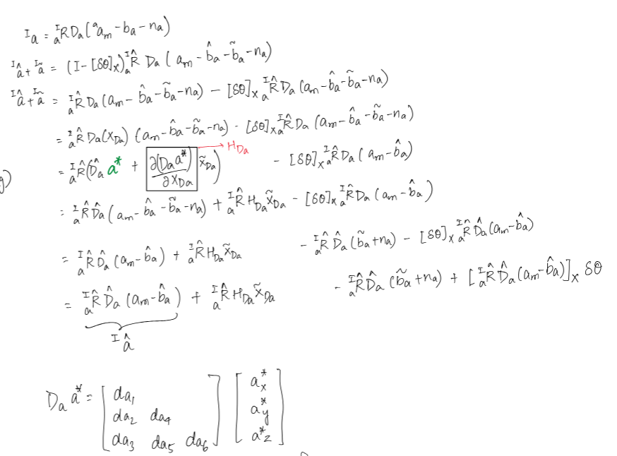
I a = I a ^ + I a ~ ≃ a I R ^ D ^ a ( a a m − b ^ a ) + a I R ^ H D a x ~ D a + ⌊ a I R ^ D ^ a ( a a m − b ^ a ) ⌋ δ θ I a − a I R ^ D ^ a b ~ a − a I R ^ D ^ a n a \begin{aligned}
{}^I\mathbf{a} &= {}^I\hat{\mathbf{a}} + {}^I\tilde{\mathbf{a}} \\
&\simeq {}^I_a\hat{\mathbf{R}}\hat{\mathbf{D}}_a \left( {}^a\mathbf{a}_m - \hat{\mathbf{b}}_a \right) + {}^I_a\hat{\mathbf{R}}\mathbf{H}_{Da}\tilde{\mathbf{x}}_{Da} \\
&+ \lfloor {}^I_a\hat{\mathbf{R}}\hat{\mathbf{D}}_a \left( {}^a\mathbf{a}_m - \hat{\mathbf{b}}_a \right) \rfloor \delta\boldsymbol{\theta}_{Ia} - {}^I_a\hat{\mathbf{R}}\hat{\mathbf{D}}_a\tilde{\mathbf{b}}_a - {}^I_a\hat{\mathbf{R}}\hat{\mathbf{D}}_a\mathbf{n}_a
\end{aligned} I a = I a ^ + I a ~ ≃ a I R ^ D ^ a ( a a m − b ^ a ) + a I R ^ H D a x ~ D a + ⌊ a I R ^ D ^ a ( a a m − b ^ a ) ⌋ δ θ I a − a I R ^ D ^ a b ~ a − a I R ^ D ^ a n a I a ^ = a I R ^ D ^ a ( a a m − b ^ a ) {}^I\hat{\mathbf{a}} = {}^I_a\hat{\mathbf{R}}\hat{\mathbf{D}}_a \left( {}^a\mathbf{a}_m - \hat{\mathbf{b}}_a \right) I a ^ = a I R ^ D ^ a ( a a m − b ^ a ) I a ~ ≃ a I R ^ H D a x ~ D a + ⌊ I a ^ ⌋ δ θ I a − a I R ^ D ^ a b ~ a − a I R ^ D ^ a n a {}^I\tilde{\mathbf{a}} \simeq {}^I_a\hat{\mathbf{R}}\mathbf{H}_{Da}\tilde{\mathbf{x}}_{Da} + \lfloor {}^I\hat{\mathbf{a}} \rfloor \delta\boldsymbol{\theta}_{Ia} - {}^I_a\hat{\mathbf{R}}\hat{\mathbf{D}}_a\tilde{\mathbf{b}}_a - {}^I_a\hat{\mathbf{R}}\hat{\mathbf{D}}_a\mathbf{n}_a I a ~ ≃ a I R ^ H D a x ~ D a + ⌊ I a ^ ⌋ δ θ I a − a I R ^ D ^ a b ~ a − a I R ^ D ^ a n a For I ω {}^I\boldsymbol{\omega} I ω I ω ~ {}^I\tilde{\boldsymbol{\omega}} I ω ~
I ω = I ω ^ + I ω ~ ≃ w I R ^ D ^ w ( w ω m − T ^ g I a ^ − b ^ g ) + ⌊ w I R ^ D ^ w ( w ω m − T ^ g I a ^ − b ^ g ) ⌋ δ θ I w + w I R ^ H D w x ~ D w − w I R ^ D ^ w ( T ^ g I a ~ + H T g x ~ T g ) − w I R ^ D ^ w ( b ~ g + n g ) \begin{aligned}
{}^I\boldsymbol{\omega} &= {}^I\hat{\boldsymbol{\omega}} + {}^I\tilde{\boldsymbol{\omega}} \\
&\simeq {}^I_w\hat{\mathbf{R}}\hat{\mathbf{D}}_w \left( {}^w\boldsymbol{\omega}_m - \hat{\mathbf{T}}_g {}^I\hat{\mathbf{a}} - \hat{\mathbf{b}}_g \right) + \lfloor {}^I_w\hat{\mathbf{R}}\hat{\mathbf{D}}_w \left( {}^w\boldsymbol{\omega}_m - \hat{\mathbf{T}}_g {}^I\hat{\mathbf{a}} - \hat{\mathbf{b}}_g \right) \rfloor \delta\boldsymbol{\theta}_{Iw} \\
&+ {}^I_w\hat{\mathbf{R}}\mathbf{H}_{Dw}\tilde{\mathbf{x}}_{Dw} - {}^I_w\hat{\mathbf{R}}\hat{\mathbf{D}}_w \left( \hat{\mathbf{T}}_g {}^I\tilde{\mathbf{a}} + \mathbf{H}_{Tg}\tilde{\mathbf{x}}_{Tg} \right) - {}^I_w\hat{\mathbf{R}}\hat{\mathbf{D}}_w \left( \tilde{\mathbf{b}}_g + \mathbf{n}_g \right)
\end{aligned} I ω = I ω ^ + I ω ~ ≃ w I R ^ D ^ w ( w ω m − T ^ g I a ^ − b ^ g ) + ⌊ w I R ^ D ^ w ( w ω m − T ^ g I a ^ − b ^ g ) ⌋ δ θ I w + w I R ^ H D w x ~ D w − w I R ^ D ^ w ( T ^ g I a ~ + H T g x ~ T g ) − w I R ^ D ^ w ( b ~ g + n g ) I ω ^ = w I R ^ D ^ w ( w ω m − T ^ g I a ^ − b ^ g ) {}^I\hat{\boldsymbol{\omega}} = {}^I_w\hat{\mathbf{R}}\hat{\mathbf{D}}_w \left( {}^w\boldsymbol{\omega}_m - \hat{\mathbf{T}}_g {}^I\hat{\mathbf{a}} - \hat{\mathbf{b}}_g \right) I ω ^ = w I R ^ D ^ w ( w ω m − T ^ g I a ^ − b ^ g ) I ω ~ ≃ − w I R ^ D ^ w b ~ g + w I R ^ D ^ w T ^ g a I R ^ D ^ a b ~ a + w I R ^ H D w x ~ D w − w I R ^ D ^ w T ^ g a I R ^ H D a x ~ D a + ⌊ I ω ^ ⌋ δ θ I w − w I R ^ D ^ w T ^ g ⌊ I a ^ ⌋ δ θ I a − w I R ^ D ^ w H T g x ~ T g − w I R ^ D ^ w n g + w I R ^ D ^ w T ^ g a I R ^ D ^ a n a \begin{aligned}
{}^I\tilde{\boldsymbol{\omega}} &\simeq -{}^I_w\hat{\mathbf{R}}\hat{\mathbf{D}}_w\tilde{\mathbf{b}}_g + {}^I_w\hat{\mathbf{R}}\hat{\mathbf{D}}_w \hat{\mathbf{T}}_g {}^I_a\hat{\mathbf{R}}\hat{\mathbf{D}}_a\tilde{\mathbf{b}}_a + {}^I_w\hat{\mathbf{R}}\mathbf{H}_{Dw}\tilde{\mathbf{x}}_{Dw} \\
&- {}^I_w\hat{\mathbf{R}}\hat{\mathbf{D}}_w \hat{\mathbf{T}}_g {}^I_a\hat{\mathbf{R}}\mathbf{H}_{Da}\tilde{\mathbf{x}}_{Da} + \lfloor {}^I\hat{\boldsymbol{\omega}} \rfloor \delta\boldsymbol{\theta}_{Iw} - {}^I_w\hat{\mathbf{R}}\hat{\mathbf{D}}_w \hat{\mathbf{T}}_g \lfloor {}^I\hat{\mathbf{a}} \rfloor \delta\boldsymbol{\theta}_{Ia} \\
&- {}^I_w\hat{\mathbf{R}}\hat{\mathbf{D}}_w \mathbf{H}_{Tg}\tilde{\mathbf{x}}_{Tg} - {}^I_w\hat{\mathbf{R}}\hat{\mathbf{D}}_w\mathbf{n}_g + {}^I_w\hat{\mathbf{R}}\hat{\mathbf{D}}_w \hat{\mathbf{T}}_g {}^I_a\hat{\mathbf{R}}\hat{\mathbf{D}}_a\mathbf{n}_a
\end{aligned} I ω ~ ≃ − w I R ^ D ^ w b ~ g + w I R ^ D ^ w T ^ g a I R ^ D ^ a b ~ a + w I R ^ H D w x ~ D w − w I R ^ D ^ w T ^ g a I R ^ H D a x ~ D a + ⌊ I ω ^ ⌋ δ θ I w − w I R ^ D ^ w T ^ g ⌊ I a ^ ⌋ δ θ I a − w I R ^ D ^ w H T g x ~ T g − w I R ^ D ^ w n g + w I R ^ D ^ w T ^ g a I R ^ D ^ a n a where we need to define H D w \mathbf{H}_{Dw} H D w H D a \mathbf{H}_{Da} H D a H T g \mathbf{H}_{Tg} H T g KALIBR model, we
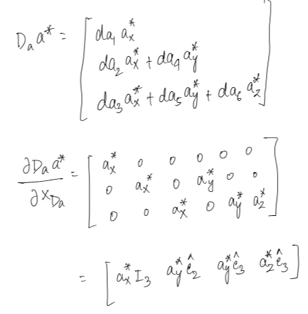
H D w = [ w w ^ 1 I 3 w w ^ 2 e 2 w w ^ 2 e 3 w w ^ 3 e 3 ] H D a = [ a a ^ 1 I 3 a a ^ 2 e 2 a a ^ 2 e 3 a a ^ 3 e 3 ] H T g = [ I a ^ 1 I 3 I a ^ 2 I 3 I a ^ 3 I 3 ] \begin{aligned}
\mathbf{H}_{Dw} &= \begin{bmatrix} {}^w\hat{w}_1\mathbf{I}_3 & {}^w\hat{w}_2\mathbf{e}_2 & {}^w\hat{w}_2\mathbf{e}_3 & {}^w\hat{w}_3\mathbf{e}_3 \end{bmatrix} \\
\mathbf{H}_{Da} &= \begin{bmatrix} {}^a\hat{a}_1\mathbf{I}_3 & {}^a\hat{a}_2\mathbf{e}_2 & {}^a\hat{a}_2\mathbf{e}_3 & {}^a\hat{a}_3\mathbf{e}_3 \end{bmatrix} \\
\mathbf{H}_{Tg} &= \begin{bmatrix} {}^I\hat{a}_1\mathbf{I}_3 & {}^I\hat{a}_2\mathbf{I}_3 & {}^I\hat{a}_3\mathbf{I}_3 \end{bmatrix}
\end{aligned} H D w H D a H T g = [ w w ^ 1 I 3 w w ^ 2 e 2 w w ^ 2 e 3 w w ^ 3 e 3 ] = [ a a ^ 1 I 3 a a ^ 2 e 2 a a ^ 2 e 3 a a ^ 3 e 3 ] = [ I a ^ 1 I 3 I a ^ 2 I 3 I a ^ 3 I 3 ] Check below for detailed derivation:
By summarizing the above equations, we have:
[ I k ω ~ I k a ~ ] = [ H b H i n ] [ x ~ b x ~ i n ] + H n [ n d g n d a ] \begin{bmatrix} {}^{I_k}\tilde{\boldsymbol{\omega}} \\ {}^{I_k}\tilde{\mathbf{a}} \end{bmatrix} = \begin{bmatrix} \mathbf{H}_b & \mathbf{H}_{in} \end{bmatrix} \begin{bmatrix} \tilde{\mathbf{x}}_b \\ \tilde{\mathbf{x}}_{in} \end{bmatrix} + \mathbf{H}_n \begin{bmatrix} \mathbf{n}_{dg} \\ \mathbf{n}_{da} \end{bmatrix} [ I k ω ~ I k a ~ ] = [ H b H in ] [ x ~ b x ~ in ] + H n [ n d g n d a ] where we have defined:
H b = H n = [ − w I R ^ D ^ w w I R ^ D ^ w T ^ g a I R ^ D ^ a 0 3 − a I R ^ D ^ a ] \mathbf{H}_b = \mathbf{H}_n = \begin{bmatrix} -{}^I_w\hat{\mathbf{R}}\hat{\mathbf{D}}_w & {}^I_w\hat{\mathbf{R}}\hat{\mathbf{D}}_w \hat{\mathbf{T}}_g {}^I_a\hat{\mathbf{R}}\hat{\mathbf{D}}_a \\ \mathbf{0}_3 & -{}^I_a\hat{\mathbf{R}}\hat{\mathbf{D}}_a \end{bmatrix} H b = H n = [ − w I R ^ D ^ w 0 3 w I R ^ D ^ w T ^ g a I R ^ D ^ a − a I R ^ D ^ a ] H i n = [ H w H a H I w H I a H g ] \mathbf{H}_{in} = \begin{bmatrix} \mathbf{H}_w & \mathbf{H}_a & \mathbf{H}_{Iw} & \mathbf{H}_{Ia} & \mathbf{H}_g \end{bmatrix} H in = [ H w H a H I w H I a H g ] H w = ∂ [ I k ω ~ I k a ~ ] ∂ x D w = [ w I R ^ H D w 0 3 ] \mathbf{H}_w = \frac{\partial [{}^{I_k}\tilde{\boldsymbol{\omega}} \,\, {}^{I_k}\tilde{\mathbf{a}}]}{\partial \mathbf{x}_{Dw}} = \begin{bmatrix} {}^I_w\hat{\mathbf{R}}\mathbf{H}_{Dw} \\ \mathbf{0}_3 \end{bmatrix} H w = ∂ x D w ∂ [ I k ω ~ I k a ~ ] = [ w I R ^ H D w 0 3 ] H a = ∂ [ I k ω ~ I k a ~ ] ∂ x D a = [ − w I R ^ D ^ w T ^ g a I R ^ H D a a I R ^ H D a ] \mathbf{H}_a = \frac{\partial [{}^{I_k}\tilde{\boldsymbol{\omega}} \,\, {}^{I_k}\tilde{\mathbf{a}}]}{\partial \mathbf{x}_{Da}} = \begin{bmatrix} -{}^I_w\hat{\mathbf{R}}\hat{\mathbf{D}}_w \hat{\mathbf{T}}_g {}^I_a\hat{\mathbf{R}}\mathbf{H}_{Da} \\ {}^I_a\hat{\mathbf{R}}\mathbf{H}_{Da} \end{bmatrix} H a = ∂ x D a ∂ [ I k ω ~ I k a ~ ] = [ − w I R ^ D ^ w T ^ g a I R ^ H D a a I R ^ H D a ] H I w = ∂ [ I k ω ~ I k a ~ ] ∂ w I δ θ = [ ⌊ I ω ^ ⌋ 0 3 ] \mathbf{H}_{Iw} = \frac{\partial [{}^{I_k}\tilde{\boldsymbol{\omega}} \,\, {}^{I_k}\tilde{\mathbf{a}}]}{\partial {}^I_w\delta\boldsymbol{\theta}} = \begin{bmatrix} \lfloor {}^I\hat{\boldsymbol{\omega}} \rfloor \\ \mathbf{0}_3 \end{bmatrix} H I w = ∂ w I δ θ ∂ [ I k ω ~ I k a ~ ] = [ ⌊ I ω ^ ⌋ 0 3 ] H I a = ∂ [ I k ω ~ I k a ~ ] ∂ a I δ θ = [ − a I R ^ D ^ w T ^ g ⌊ I a ^ ⌋ ⌊ I a ^ ⌋ ] \mathbf{H}_{Ia} = \frac{\partial [{}^{I_k}\tilde{\boldsymbol{\omega}} \,\, {}^{I_k}\tilde{\mathbf{a}}]}{\partial {}^I_a\delta\boldsymbol{\theta}} = \begin{bmatrix} -{}^I_a\hat{\mathbf{R}}\hat{\mathbf{D}}_w \hat{\mathbf{T}}_g \lfloor {}^I\hat{\mathbf{a}} \rfloor \\ \lfloor {}^I\hat{\mathbf{a}} \rfloor \end{bmatrix} H I a = ∂ a I δ θ ∂ [ I k ω ~ I k a ~ ] = [ − a I R ^ D ^ w T ^ g ⌊ I a ^ ⌋ ⌊ I a ^ ⌋ ] H g = ∂ [ I k ω ~ I k a ~ ] ∂ x T g = [ − w I R ^ D ^ w H T g 0 3 ] \mathbf{H}_g = \frac{\partial [{}^{I_k}\tilde{\boldsymbol{\omega}} \,\, {}^{I_k}\tilde{\mathbf{a}}]}{\partial \mathbf{x}_{Tg}} = \begin{bmatrix} -{}^I_w\hat{\mathbf{R}}\hat{\mathbf{D}}_w \mathbf{H}_{Tg} \\ \mathbf{0}_3 \end{bmatrix} H g = ∂ x T g ∂ [ I k ω ~ I k a ~ ] = [ − w I R ^ D ^ w H T g 0 3 ] We then linearize Δ R k , Δ p k \Delta\mathbf{R}_k, \Delta\mathbf{p}_k Δ R k , Δ p k Δ v k \Delta\mathbf{v}_k Δ v k Δ R k \Delta\mathbf{R}_k Δ R k
Δ R k = exp ( − I k ω Δ t k ) = exp ( − ( I k ω ^ + I k ω ~ ) Δ t k ) ≃ exp ( − I k ω ^ Δ t k ) ⋅ exp ( − J r ( − I k ω ^ Δ t k ) I k ω ~ Δ t k ) ≃ exp ( − Δ R ^ k J r ( − I k ω ^ Δ t k ) I k ω ~ Δ t k ) ⏟ Δ R ~ k exp ( − I k ω ^ Δ t k ) \begin{aligned}
\Delta\mathbf{R}_k &= \exp(-{}^{I_k}\boldsymbol{\omega}\Delta t_k) \\
&= \exp(-({}^{I_k}\hat{\boldsymbol{\omega}} + {}^{I_k}\tilde{\boldsymbol{\omega}})\Delta t_k) \\
&\simeq \exp(-{}^{I_k}\hat{\boldsymbol{\omega}}\Delta t_k) \cdot \exp(-\mathbf{J}_r(-{}^{I_k}\hat{\boldsymbol{\omega}}\Delta t_k){}^{I_k}\tilde{\boldsymbol{\omega}}\Delta t_k) \\
&\simeq \underbrace{\exp(-\Delta\hat{\mathbf{R}}_k \mathbf{J}_r(-{}^{I_k}\hat{\boldsymbol{\omega}}\Delta t_k){}^{I_k}\tilde{\boldsymbol{\omega}}\Delta t_k)}_{\Delta\tilde{\mathbf{R}}_k} \exp(-{}^{I_k}\hat{\boldsymbol{\omega}}\Delta t_k)
\end{aligned} Δ R k = exp ( − I k ω Δ t k ) = exp ( − ( I k ω ^ + I k ω ~ ) Δ t k ) ≃ exp ( − I k ω ^ Δ t k ) ⋅ exp ( − J r ( − I k ω ^ Δ t k ) I k ω ~ Δ t k ) ≃ Δ R ~ k exp ( − Δ R ^ k J r ( − I k ω ^ Δ t k ) I k ω ~ Δ t k ) exp ( − I k ω ^ Δ t k ) For the integration of Δ p k \Delta\mathbf{p}_k Δ p k
Δ p k = ∫ t k t k + 1 ∫ t k s exp ( I k ω δ τ ) d τ d s ⋅ I k a = ∫ t k t k + 1 ∫ t k s exp ( ( I k ω ^ + I k ω ~ ) δ τ ) d τ d s ⋅ ( I k a ^ + I k a ~ ) ≃ ∫ t k t k + 1 ∫ t k s exp ( I k ω ^ δ τ ) exp ( J r ( I k ω ^ δ τ ) I k ω ~ δ τ ) d τ d s ⋅ ( I k a ^ + I k a ~ ) ≃ ∫ t k t k + 1 ∫ t k s exp ( I k ω ^ δ τ ) ( I + ⌊ J r ( I k ω ^ δ τ ) I k ω ~ δ τ ⌋ ) d τ d s ⋅ ( I k a ^ + I k a ~ ) \begin{aligned}
\Delta\mathbf{p}_k &= \int_{t_k}^{t_{k+1}} \int_{t_k}^{s} \exp({}^{I_k}\boldsymbol{\omega}\delta\tau) d\tau ds \cdot {}^{I_k}\mathbf{a} \\
&= \int_{t_k}^{t_{k+1}} \int_{t_k}^{s} \exp(({}^{I_k}\hat{\boldsymbol{\omega}} + {}^{I_k}\tilde{\boldsymbol{\omega}})\delta\tau) d\tau ds \cdot ({}^{I_k}\hat{\mathbf{a}} + {}^{I_k}\tilde{\mathbf{a}}) \\
&\simeq \int_{t_k}^{t_{k+1}} \int_{t_k}^{s} \exp({}^{I_k}\hat{\boldsymbol{\omega}}\delta\tau) \exp(\mathbf{J}_r({}^{I_k}\hat{\boldsymbol{\omega}}\delta\tau){}^{I_k}\tilde{\boldsymbol{\omega}}\delta\tau) d\tau ds \cdot ({}^{I_k}\hat{\mathbf{a}} + {}^{I_k}\tilde{\mathbf{a}}) \\
&\simeq \int_{t_k}^{t_{k+1}} \int_{t_k}^{s} \exp({}^{I_k}\hat{\boldsymbol{\omega}}\delta\tau) (\mathbf{I} + \lfloor \mathbf{J}_r({}^{I_k}\hat{\boldsymbol{\omega}}\delta\tau){}^{I_k}\tilde{\boldsymbol{\omega}}\delta\tau \rfloor ) d\tau ds \cdot ({}^{I_k}\hat{\mathbf{a}} + {}^{I_k}\tilde{\mathbf{a}})
\end{aligned} Δ p k = ∫ t k t k + 1 ∫ t k s exp ( I k ω δ τ ) d τ d s ⋅ I k a = ∫ t k t k + 1 ∫ t k s exp (( I k ω ^ + I k ω ~ ) δ τ ) d τ d s ⋅ ( I k a ^ + I k a ~ ) ≃ ∫ t k t k + 1 ∫ t k s exp ( I k ω ^ δ τ ) exp ( J r ( I k ω ^ δ τ ) I k ω ~ δ τ ) d τ d s ⋅ ( I k a ^ + I k a ~ ) ≃ ∫ t k t k + 1 ∫ t k s exp ( I k ω ^ δ τ ) ( I + ⌊ J r ( I k ω ^ δ τ ) I k ω ~ δ τ ⌋) d τ d s ⋅ ( I k a ^ + I k a ~ ) ≃ ∫ t k t k + 1 ∫ t k s exp ( I k ω ^ δ τ ) d τ d s ⏟ Ξ 2 ⋅ I k a ^ − ∫ t k t k + 1 ∫ t k s exp ( I k ω ^ δ τ ) ⌊ I k a ^ ⌋ J r ( I k ω ^ δ τ ) d τ d s ⏟ Ξ 4 ⋅ I k ω ~ + ∫ t k t k + 1 ∫ t k s exp ( I k ω ^ δ τ ) d τ d s ⏟ Ξ 2 ⋅ I k a ~ \begin{aligned}
&\simeq \underbrace{\int_{t_k}^{t_{k+1}} \int_{t_k}^{s} \exp({}^{I_k}\hat{\boldsymbol{\omega}}\delta\tau) d\tau ds}_{\boldsymbol{\Xi}_2} \cdot {}^{I_k}\hat{\mathbf{a}} \\
&- \underbrace{\int_{t_k}^{t_{k+1}} \int_{t_k}^{s} \exp({}^{I_k}\hat{\boldsymbol{\omega}}\delta\tau) \lfloor {}^{I_k}\hat{\mathbf{a}} \rfloor \mathbf{J}_r({}^{I_k}\hat{\boldsymbol{\omega}}\delta\tau) d\tau ds}_{\boldsymbol{\Xi}_4} \cdot {}^{I_k}\tilde{\boldsymbol{\omega}} \\
&+ \underbrace{\int_{t_k}^{t_{k+1}} \int_{t_k}^{s} \exp({}^{I_k}\hat{\boldsymbol{\omega}}\delta\tau) d\tau ds}_{\boldsymbol{\Xi}_2} \cdot {}^{I_k}\tilde{\mathbf{a}}
\end{aligned} ≃ Ξ 2 ∫ t k t k + 1 ∫ t k s exp ( I k ω ^ δ τ ) d τ d s ⋅ I k a ^ − Ξ 4 ∫ t k t k + 1 ∫ t k s exp ( I k ω ^ δ τ ) ⌊ I k a ^ ⌋ J r ( I k ω ^ δ τ ) d τ d s ⋅ I k ω ~ + Ξ 2 ∫ t k t k + 1 ∫ t k s exp ( I k ω ^ δ τ ) d τ d s ⋅ I k a ~ = Δ p ^ k − Ξ 4 I k ω ~ + Ξ 2 I k a ~ ⏟ Δ p ~ k = \Delta\hat{\mathbf{p}}_k \underbrace{- \boldsymbol{\Xi}_4 {}^{I_k}\tilde{\boldsymbol{\omega}} + \boldsymbol{\Xi}_2 {}^{I_k}\tilde{\mathbf{a}}}_{\Delta\tilde{\mathbf{p}}_k} = Δ p ^ k Δ p ~ k − Ξ 4 I k ω ~ + Ξ 2 I k a ~ = Δ p ^ k + Δ p ~ k = \Delta\hat{\mathbf{p}}_k + \Delta\tilde{\mathbf{p}}_k = Δ p ^ k + Δ p ~ k For the integration of Δ v k \Delta \mathbf{v}_k Δ v k
Δ v k = ∫ t k t k + 1 exp ( I k ω δ τ ) d τ ⋅ I k a = ∫ t k t k + 1 exp ( ( I k ω ^ + I k ω ~ ) δ τ ) d τ ⋅ ( I k a ^ + I k a ~ ) ≃ ∫ t k t k + 1 exp ( I k ω ^ δ τ ) exp ( J r ( I k ω ^ δ τ ) I k ω ~ δ τ ) d τ ⋅ ( I k a ^ + I k a ~ ) ≃ ∫ t k t k + 1 exp ( I k ω ^ δ τ ) ( I + ⌊ J r ( I k ω ^ δ τ ) I k ω ~ δ τ ⌋ ) d τ ⋅ ( I k a ^ + I k a ~ ) ≃ ∫ t k t k + 1 exp ( I k ω ^ δ τ ) d τ ⏟ Ξ 1 ⋅ I k a ^ − ∫ t k t k + 1 exp ( I k ω ^ δ τ ) ⌊ I k a ^ ⌋ J r ( I k ω ^ δ τ ) d τ ⏟ Ξ 3 ⋅ I k ω ~ + ∫ t k t k + 1 exp ( I k ω ^ δ τ ) d τ ⏟ Ξ 1 ⋅ I k a ~ \begin{aligned}
\Delta \mathbf{v}_k &= \int_{t_k}^{t_{k+1}} \exp({}^{I_k}\boldsymbol{\omega}\delta\tau) d\tau \cdot {}^{I_k}\mathbf{a} \\
&= \int_{t_k}^{t_{k+1}} \exp(({}^{I_k}\hat{\boldsymbol{\omega}} + {}^{I_k}\tilde{\boldsymbol{\omega}})\delta\tau) d\tau \cdot ({}^{I_k}\hat{\mathbf{a}} + {}^{I_k}\tilde{\mathbf{a}}) \\
&\simeq \int_{t_k}^{t_{k+1}} \exp({}^{I_k}\hat{\boldsymbol{\omega}}\delta\tau) \exp(\mathbf{J}_r({}^{I_k}\hat{\boldsymbol{\omega}}\delta\tau){}^{I_k}\tilde{\boldsymbol{\omega}}\delta\tau) d\tau \cdot ({}^{I_k}\hat{\mathbf{a}} + {}^{I_k}\tilde{\mathbf{a}}) \\
&\simeq \int_{t_k}^{t_{k+1}} \exp({}^{I_k}\hat{\boldsymbol{\omega}}\delta\tau) (\mathbf{I} + \lfloor \mathbf{J}_r({}^{I_k}\hat{\boldsymbol{\omega}}\delta\tau){}^{I_k}\tilde{\boldsymbol{\omega}}\delta\tau \rfloor ) d\tau \cdot ({}^{I_k}\hat{\mathbf{a}} + {}^{I_k}\tilde{\mathbf{a}}) \\
&\simeq \underbrace{\int_{t_k}^{t_{k+1}} \exp({}^{I_k}\hat{\boldsymbol{\omega}}\delta\tau) d\tau}_{\boldsymbol{\Xi}_1} \cdot {}^{I_k}\hat{\mathbf{a}} \\
&- \underbrace{\int_{t_k}^{t_{k+1}} \exp({}^{I_k}\hat{\boldsymbol{\omega}}\delta\tau) \lfloor {}^{I_k}\hat{\mathbf{a}} \rfloor \mathbf{J}_r({}^{I_k}\hat{\boldsymbol{\omega}}\delta\tau) d\tau}_{\boldsymbol{\Xi}_3} \cdot {}^{I_k}\tilde{\boldsymbol{\omega}} \\
&+ \underbrace{\int_{t_k}^{t_{k+1}} \exp({}^{I_k}\hat{\boldsymbol{\omega}}\delta\tau) d\tau}_{\boldsymbol{\Xi}_1} \cdot {}^{I_k}\tilde{\mathbf{a}}
\end{aligned} Δ v k = ∫ t k t k + 1 exp ( I k ω δ τ ) d τ ⋅ I k a = ∫ t k t k + 1 exp (( I k ω ^ + I k ω ~ ) δ τ ) d τ ⋅ ( I k a ^ + I k a ~ ) ≃ ∫ t k t k + 1 exp ( I k ω ^ δ τ ) exp ( J r ( I k ω ^ δ τ ) I k ω ~ δ τ ) d τ ⋅ ( I k a ^ + I k a ~ ) ≃ ∫ t k t k + 1 exp ( I k ω ^ δ τ ) ( I + ⌊ J r ( I k ω ^ δ τ ) I k ω ~ δ τ ⌋) d τ ⋅ ( I k a ^ + I k a ~ ) ≃ Ξ 1 ∫ t k t k + 1 exp ( I k ω ^ δ τ ) d τ ⋅ I k a ^ − Ξ 3 ∫ t k t k + 1 exp ( I k ω ^ δ τ ) ⌊ I k a ^ ⌋ J r ( I k ω ^ δ τ ) d τ ⋅ I k ω ~ + Ξ 1 ∫ t k t k + 1 exp ( I k ω ^ δ τ ) d τ ⋅ I k a ~ = Δ v ^ k − Ξ 3 I k ω ~ + Ξ 1 I k a ~ ⏟ Δ v ~ k = \Delta \hat{\mathbf{v}}_k \underbrace{- \boldsymbol{\Xi}_3 {}^{I_k}\tilde{\boldsymbol{\omega}} + \boldsymbol{\Xi}_1 {}^{I_k}\tilde{\mathbf{a}}}_{\Delta \tilde{\mathbf{v}}_k} = Δ v ^ k Δ v ~ k − Ξ 3 I k ω ~ + Ξ 1 I k a ~ = Δ v ^ k + Δ v ~ k = \Delta \hat{\mathbf{v}}_k + \Delta \tilde{\mathbf{v}}_k = Δ v ^ k + Δ v ~ k where δ τ = t τ − t k \delta\tau = t_\tau - t_k δ τ = t τ − t k Ξ i , i = 1 … 4 \boldsymbol{\Xi}_i, i = 1 \dots 4 Ξ i , i = 1 … 4 Integration Component Definitions section. J r ( − I k ω ^ Δ t k ) \mathbf{J}_r(-{}^{I_k}\hat{\boldsymbol{\omega}}\Delta t_k) J r ( − I k ω ^ Δ t k ) S O ( 3 ) SO(3) SO ( 3 ) Integration Component Definitions ):
Δ R k = Δ R ~ k Δ R ^ k ≜ exp ( − Δ R ^ k J r ( Δ θ k ) I k ω ~ Δ t k ) Δ R ^ k \Delta\mathbf{R}_k = \Delta\tilde{\mathbf{R}}_k\Delta\hat{\mathbf{R}}_k \triangleq \exp\left(-\Delta\hat{\mathbf{R}}_k\mathbf{J}_r(\Delta\boldsymbol{\theta}_k){}^{I_k}\tilde{\boldsymbol{\omega}}\Delta t_k\right) \Delta\hat{\mathbf{R}}_k Δ R k = Δ R ~ k Δ R ^ k ≜ exp ( − Δ R ^ k J r ( Δ θ k ) I k ω ~ Δ t k ) Δ R ^ k Δ p k = Δ p ^ k + Δ p ~ k ≜ Δ p ^ k − Ξ 4 I k ω ~ + Ξ 2 I k a ~ \Delta\mathbf{p}_k = \Delta\hat{\mathbf{p}}_k + \Delta\tilde{\mathbf{p}}_k \triangleq \Delta\hat{\mathbf{p}}_k - \boldsymbol{\Xi}_4 {}^{I_k}\tilde{\boldsymbol{\omega}} + \boldsymbol{\Xi}_2 {}^{I_k}\tilde{\mathbf{a}} Δ p k = Δ p ^ k + Δ p ~ k ≜ Δ p ^ k − Ξ 4 I k ω ~ + Ξ 2 I k a ~ Δ v k = Δ v ^ k + Δ v ~ k ≜ Δ v ^ k − Ξ 3 I k ω ~ + Ξ 1 I k a ~ \Delta\mathbf{v}_k = \Delta\hat{\mathbf{v}}_k + \Delta\tilde{\mathbf{v}}_k \triangleq \Delta\hat{\mathbf{v}}_k - \boldsymbol{\Xi}_3 {}^{I_k}\tilde{\boldsymbol{\omega}} + \boldsymbol{\Xi}_1 {}^{I_k}\tilde{\mathbf{a}} Δ v k = Δ v ^ k + Δ v ~ k ≜ Δ v ^ k − Ξ 3 I k ω ~ + Ξ 1 I k a ~ where J r ( Δ θ k ) ≜ J r ( − I k ω ^ k Δ t k ) \mathbf{J}_r(\Delta\boldsymbol{\theta}_k) \triangleq \mathbf{J}_r(-{}^{I_k}\hat{\boldsymbol{\omega}}_k\Delta t_k) J r ( Δ θ k ) ≜ J r ( − I k ω ^ k Δ t k ) Ξ 3 \boldsymbol{\Xi}_3 Ξ 3 Ξ 4 \boldsymbol{\Xi}_4 Ξ 4
Ξ 3 = ∫ t k t k + 1 I τ I k R ⌊ I τ a ⌋ J r ( I k ω ^ k δ τ ) δ τ d τ \boldsymbol{\Xi}_3 = \int_{t_k}^{t_{k+1}} {}^{I_k}_{I_\tau}\mathbf{R} \lfloor {}^{I_\tau}\mathbf{a} \rfloor \mathbf{J}_r({}^{I_k}\hat{\boldsymbol{\omega}}_k \delta\tau) \delta\tau \, d\tau Ξ 3 = ∫ t k t k + 1 I τ I k R ⌊ I τ a ⌋ J r ( I k ω ^ k δ τ ) δ τ d τ Ξ 4 = ∫ t k t k + 1 ∫ t k s I τ I k R ⌊ I τ a ⌋ J r ( I k ω ^ k δ τ ) δ τ d τ d s \boldsymbol{\Xi}_4 = \int_{t_k}^{t_{k+1}} \int_{t_k}^{s} {}^{I_k}_{I_\tau}\mathbf{R} \lfloor {}^{I_\tau}\mathbf{a} \rfloor \mathbf{J}_r({}^{I_k}\hat{\boldsymbol{\omega}}_k \delta\tau) \delta\tau \, d\tau ds Ξ 4 = ∫ t k t k + 1 ∫ t k s I τ I k R ⌊ I τ a ⌋ J r ( I k ω ^ k δ τ ) δ τ d τ d s Nominal state Kinematics ¶ Under the assumption of constant I k ω ^ {}^{I_k}\hat{\boldsymbol{\omega}} I k ω ^ I k a ^ {}^{I_k}\hat{\mathbf{a}} I k a ^ t k + 1 t_{k+1} t k + 1
G I k + 1 R ^ ≃ Δ R k G I k R ^ {}^{I_{k+1}}_G\hat{\mathbf{R}} \simeq \Delta\mathbf{R}_k {}^{I_k}_G\hat{\mathbf{R}} G I k + 1 R ^ ≃ Δ R k G I k R ^ G p ^ I k + 1 ≃ G p ^ I k + G v ^ I k Δ t k + G I k R ^ ⊤ Ξ 2 I k a ^ − 1 2 G g Δ t k 2 {}^G\hat{\mathbf{p}}_{I_{k+1}} \simeq {}^G\hat{\mathbf{p}}_{I_k} + {}^G\hat{\mathbf{v}}_{I_k}\Delta t_k + {}_G^{I_k}\hat{\mathbf{R}}^\top \boldsymbol{\Xi}_2 {}^{I_k}\hat{\mathbf{a}} - \frac{1}{2}{}^G\mathbf{g}\Delta t_k^2 G p ^ I k + 1 ≃ G p ^ I k + G v ^ I k Δ t k + G I k R ^ ⊤ Ξ 2 I k a ^ − 2 1 G g Δ t k 2 G v ^ I k + 1 ≃ G v ^ I k + G I k R ^ ⊤ Ξ 1 I k a ^ − G g Δ t k {}^G\hat{\mathbf{v}}_{I_{k+1}} \simeq {}^G\hat{\mathbf{v}}_{I_k} + {}_G^{I_k}\hat{\mathbf{R}}^\top \boldsymbol{\Xi}_1 {}^{I_k}\hat{\mathbf{a}} - {}^G\mathbf{g}\Delta t_k G v ^ I k + 1 ≃ G v ^ I k + G I k R ^ ⊤ Ξ 1 I k a ^ − G g Δ t k b ^ g k + 1 = b ^ g k \hat{\mathbf{b}}_{g_{k+1}} = \hat{\mathbf{b}}_{g_k} b ^ g k + 1 = b ^ g k b ^ a k + 1 = b ^ a k \hat{\mathbf{b}}_{a_{k+1}} = \hat{\mathbf{b}}_{a_k} b ^ a k + 1 = b ^ a k Error state Kinematics ¶ Hence, the linearized IMU system is:
δ θ k + 1 ≃ Δ R ^ k δ θ k + Δ R ^ k J r ( Δ θ k ) Δ t k I k ω ~ \delta\boldsymbol{\theta}_{k+1} \simeq \Delta\hat{\mathbf{R}}_k \delta\boldsymbol{\theta}_k + \Delta\hat{\mathbf{R}}_k \mathbf{J}_r(\Delta\boldsymbol{\theta}_k) \Delta t_k {}^{I_k}\tilde{\boldsymbol{\omega}} δ θ k + 1 ≃ Δ R ^ k δ θ k + Δ R ^ k J r ( Δ θ k ) Δ t k I k ω ~ G p ~ I k + 1 ≃ G p ~ I k + G v ~ I k Δ t k − G I R ^ ⊤ ⌊ Δ p ^ k ⌋ δ θ k + G I R ^ ⊤ ( − Ξ 4 I k ω ~ + Ξ 2 I k a ~ ) {}^G\tilde{\mathbf{p}}_{I_{k+1}} \simeq {}^G\tilde{\mathbf{p}}_{I_k} + {}^G\tilde{\mathbf{v}}_{I_k}\Delta t_k - {}^I_G\hat{\mathbf{R}}^\top \lfloor \Delta\hat{\mathbf{p}}_k \rfloor \delta\boldsymbol{\theta}_k + {}^I_G\hat{\mathbf{R}}^\top \left( -\boldsymbol{\Xi}_4 {}^{I_k}\tilde{\boldsymbol{\omega}} + \boldsymbol{\Xi}_2 {}^{I_k}\tilde{\mathbf{a}} \right) G p ~ I k + 1 ≃ G p ~ I k + G v ~ I k Δ t k − G I R ^ ⊤ ⌊ Δ p ^ k ⌋ δ θ k + G I R ^ ⊤ ( − Ξ 4 I k ω ~ + Ξ 2 I k a ~ ) G v ~ I k + 1 ≃ G v ~ I k − G I R ^ ⊤ ⌊ Δ v ^ k ⌋ δ θ k + G I R ^ ⊤ ( − Ξ 3 I k ω ~ + Ξ 1 I k a ~ ) {}^G\tilde{\mathbf{v}}_{I_{k+1}} \simeq {}^G\tilde{\mathbf{v}}_{I_k} - {}^I_G\hat{\mathbf{R}}^\top \lfloor \Delta\hat{\mathbf{v}}_k \rfloor \delta\boldsymbol{\theta}_k + {}^I_G\hat{\mathbf{R}}^\top \left( -\boldsymbol{\Xi}_3 {}^{I_k}\tilde{\boldsymbol{\omega}} + \boldsymbol{\Xi}_1 {}^{I_k}\tilde{\mathbf{a}} \right) G v ~ I k + 1 ≃ G v ~ I k − G I R ^ ⊤ ⌊ Δ v ^ k ⌋ δ θ k + G I R ^ ⊤ ( − Ξ 3 I k ω ~ + Ξ 1 I k a ~ ) The overall linearized error state system is:
x ~ I k + 1 ≃ Φ I ( k + 1 , k ) x ~ I k + G I k n d k \tilde{\mathbf{x}}_{I_{k+1}} \simeq \boldsymbol{\Phi}_{I(k+1,k)}\tilde{\mathbf{x}}_{I_k} + \mathbf{G}_{Ik}\mathbf{n}_{dk} x ~ I k + 1 ≃ Φ I ( k + 1 , k ) x ~ I k + G I k n d k Φ I ( k + 1 , k ) = [ Φ n n Φ w a H b Φ w a H i n 0 6 × 9 I 6 0 6 × 24 0 24 × 9 0 24 × 6 I 24 ] \boldsymbol{\Phi}_{I(k+1,k)} = \begin{bmatrix} \boldsymbol{\Phi}_{nn} & \boldsymbol{\Phi}_{wa}\mathbf{H}_b & \boldsymbol{\Phi}_{wa}\mathbf{H}_{in} \\ \mathbf{0}_{6 \times 9} & \mathbf{I}_6 & \mathbf{0}_{6 \times 24} \\ \mathbf{0}_{24 \times 9} & \mathbf{0}_{24 \times 6} & \mathbf{I}_{24} \end{bmatrix} Φ I ( k + 1 , k ) = ⎣ ⎡ Φ nn 0 6 × 9 0 24 × 9 Φ w a H b I 6 0 24 × 6 Φ w a H in 0 6 × 24 I 24 ⎦ ⎤ G I k = [ Φ w a H n 0 9 × 6 0 6 I 6 Δ t k 0 24 × 6 0 24 × 6 ] \mathbf{G}_{Ik} = \begin{bmatrix} \boldsymbol{\Phi}_{wa}\mathbf{H}_n & \mathbf{0}_{9 \times 6} \\ \mathbf{0}_6 & \mathbf{I}_6 \Delta t_k \\ \mathbf{0}_{24 \times 6} & \mathbf{0}_{24 \times 6} \end{bmatrix} G I k = ⎣ ⎡ Φ w a H n 0 6 0 24 × 6 0 9 × 6 I 6 Δ t k 0 24 × 6 ⎦ ⎤ where Φ I ( k + 1 , k ) \boldsymbol{\Phi}_{I(k+1,k)} Φ I ( k + 1 , k ) G I k \mathbf{G}_{Ik} G I k H b \mathbf{H}_b H b H i n \mathbf{H}_{in} H in H n \mathbf{H}_n H n n d k = [ n d g ⊤ n d a ⊤ n d w g ⊤ n d w a ⊤ ] ⊤ \mathbf{n}_{dk} = [\mathbf{n}_{dg}^\top \,\, \mathbf{n}_{da}^\top \,\, \mathbf{n}_{dwg}^\top \,\, \mathbf{n}_{dwa}^\top]^\top n d k = [ n d g ⊤ n d a ⊤ n d w g ⊤ n d w a ⊤ ] ⊤ Φ n n \boldsymbol{\Phi}_{nn} Φ nn Φ w a \boldsymbol{\Phi}_{wa} Φ w a
Φ n n = [ Δ R ^ k 0 3 0 3 − G I R ^ ⊤ ⌊ Δ p ^ k ⌋ I 3 I 3 Δ t k − G I R ^ ⊤ ⌊ Δ v ^ k ⌋ 0 3 I 3 ] \boldsymbol{\Phi}_{nn} = \begin{bmatrix} \Delta\hat{\mathbf{R}}_k & \mathbf{0}_3 & \mathbf{0}_3 \\ -{}^I_G\hat{\mathbf{R}}^\top \lfloor \Delta\hat{\mathbf{p}}_k \rfloor & \mathbf{I}_3 & \mathbf{I}_3 \Delta t_k \\ -{}^I_G\hat{\mathbf{R}}^\top \lfloor \Delta\hat{\mathbf{v}}_k \rfloor & \mathbf{0}_3 & \mathbf{I}_3 \end{bmatrix} Φ nn = ⎣ ⎡ Δ R ^ k − G I R ^ ⊤ ⌊ Δ p ^ k ⌋ − G I R ^ ⊤ ⌊ Δ v ^ k ⌋ 0 3 I 3 0 3 0 3 I 3 Δ t k I 3 ⎦ ⎤ Φ w a = [ Δ R ^ k J r ( Δ θ k ) Δ t k 0 3 − G I R ^ ⊤ Ξ 4 G I R ^ ⊤ Ξ 2 − G I R ^ ⊤ Ξ 3 G I R ^ ⊤ Ξ 1 ] \boldsymbol{\Phi}_{wa} = \begin{bmatrix} \Delta\hat{\mathbf{R}}_k \mathbf{J}_r(\Delta\boldsymbol{\theta}_k)\Delta t_k & \mathbf{0}_3 \\ -{}^I_G\hat{\mathbf{R}}^\top \boldsymbol{\Xi}_4 & {}^I_G\hat{\mathbf{R}}^\top \boldsymbol{\Xi}_2 \\ -{}^I_G\hat{\mathbf{R}}^\top \boldsymbol{\Xi}_3 & {}^I_G\hat{\mathbf{R}}^\top \boldsymbol{\Xi}_1 \end{bmatrix} Φ w a = ⎣ ⎡ Δ R ^ k J r ( Δ θ k ) Δ t k − G I R ^ ⊤ Ξ 4 − G I R ^ ⊤ Ξ 3 0 3 G I R ^ ⊤ Ξ 2 G I R ^ ⊤ Ξ 1 ⎦ ⎤ Note that n d ∗ ∼ N ( 0 , σ ∗ 2 I 3 Δ t k ) \mathbf{n}_{d*} \sim \mathcal{N}(\mathbf{0}, \frac{\sigma_*^2 \mathbf{I}_3}{\Delta t_k}) n d ∗ ∼ N ( 0 , Δ t k σ ∗ 2 I 3 ) n d I \mathbf{n}_{dI} n d I
Q d I = [ σ g 2 Δ t k I 3 0 3 0 3 0 3 0 3 σ a 2 Δ t k I 3 0 3 0 3 0 3 0 3 σ w g 2 Δ t k I 3 0 3 0 3 0 3 0 3 σ w a 2 Δ t k I 3 ] \mathbf{Q}_{dI} = \begin{bmatrix} \frac{\sigma_g^2}{\Delta t_k}\mathbf{I}_3 & \mathbf{0}_3 & \mathbf{0}_3 & \mathbf{0}_3 \\ \mathbf{0}_3 & \frac{\sigma_a^2}{\Delta t_k}\mathbf{I}_3 & \mathbf{0}_3 & \mathbf{0}_3 \\ \mathbf{0}_3 & \mathbf{0}_3 & \sigma_{wg}^2\Delta t_k \mathbf{I}_3 & \mathbf{0}_3 \\ \mathbf{0}_3 & \mathbf{0}_3 & \mathbf{0}_3 & \sigma_{wa}^2\Delta t_k \mathbf{I}_3 \end{bmatrix} Q d I = ⎣ ⎡ Δ t k σ g 2 I 3 0 3 0 3 0 3 0 3 Δ t k σ a 2 I 3 0 3 0 3 0 3 0 3 σ w g 2 Δ t k I 3 0 3 0 3 0 3 0 3 σ w a 2 Δ t k I 3 ⎦ ⎤ Finally, the covariance propagation can be derived as:
P k + 1 = Φ I ( k + 1 , k ) P k Φ I ( k + 1 , k ) ⊤ + G I k Q d I G I k ⊤ \mathbf{P}_{k+1} = \boldsymbol{\Phi}_{I(k+1,k)} \mathbf{P}_k \boldsymbol{\Phi}_{I(k+1,k)}^\top + \mathbf{G}_{Ik} \mathbf{Q}_{dI} \mathbf{G}_{Ik}^\top P k + 1 = Φ I ( k + 1 , k ) P k Φ I ( k + 1 , k ) ⊤ + G I k Q d I G I k ⊤ Integration Component Definitions ¶ When deriving the components, we drop the subscripts for simplicity. As we define angular velocity ω ^ = ∣ ∣ I ω ^ ∣ ∣ \hat{\omega} = || {}^I\hat{\boldsymbol{\omega}} || ω ^ = ∣∣ I ω ^ ∣∣ k = I ω ^ / ∣ ∣ I ω ^ ∣ ∣ \mathbf{k} = {}^I\hat{\boldsymbol{\omega}} / || {}^I\hat{\boldsymbol{\omega}} || k = I ω ^ /∣∣ I ω ^ ∣∣ δ t \delta t δ t
Ξ 1 = I 3 δ t + 1 − cos ( ω ^ δ t ) ω ^ ⌊ k ^ ⌋ + ( δ t − sin ( ω ^ δ t ) ω ^ ) ⌊ k ^ ⌋ 2 \boldsymbol{\Xi}_1 = \mathbf{I}_3 \delta t + \frac{1 - \cos(\hat{\omega} \delta t)}{\hat{\omega}} \lfloor \hat{\mathbf{k}} \rfloor + \left( \delta t - \frac{\sin(\hat{\omega} \delta t)}{\hat{\omega}} \right) \lfloor \hat{\mathbf{k}} \rfloor^2 Ξ 1 = I 3 δ t + ω ^ 1 − cos ( ω ^ δ t ) ⌊ k ^ ⌋ + ( δ t − ω ^ sin ( ω ^ δ t ) ) ⌊ k ^ ⌋ 2 The second integration we need is:
Ξ 2 = 1 2 δ t 2 I 3 + ω ^ δ t − sin ( ω ^ δ t ) ω ^ 2 ⌊ k ^ ⌋ + ( 1 2 δ t 2 − 1 − cos ( ω ^ δ t ) ω ^ 2 ) ⌊ k ^ ⌋ 2 \boldsymbol{\Xi}_2 = \frac{1}{2} \delta t^2 \mathbf{I}_3 + \frac{\hat{\omega} \delta t - \sin(\hat{\omega} \delta t)}{\hat{\omega}^2} \lfloor \hat{\mathbf{k}} \rfloor + \left( \frac{1}{2} \delta t^2 - \frac{1 - \cos(\hat{\omega} \delta t)}{\hat{\omega}^2} \right) \lfloor \hat{\mathbf{k}} \rfloor^2 Ξ 2 = 2 1 δ t 2 I 3 + ω ^ 2 ω ^ δ t − sin ( ω ^ δ t ) ⌊ k ^ ⌋ + ( 2 1 δ t 2 − ω ^ 2 1 − cos ( ω ^ δ t ) ) ⌊ k ^ ⌋ 2 The third integration can be written as:
Ξ 3 = 1 2 δ t 2 ⌊ a ^ ⌋ + sin ( ω ^ δ t i ) − ω ^ δ t ω ^ 2 ⌊ a ^ ⌋ ⌊ k ^ ⌋ + sin ( ω ^ δ t ) − ω ^ δ t cos ( ω ^ δ t ) ω ^ 2 ⌊ k ^ ⌋ ⌊ a ^ ⌋ + ( 1 2 δ t 2 − 1 − cos ( ω ^ δ t ) ω ^ 2 ) ⌊ a ^ ⌋ ⌊ k ^ ⌋ 2 + ( 1 2 δ t 2 + 1 − cos ( ω ^ δ t ) − ω ^ δ t sin ( ω ^ δ t ) ω ^ 2 ) ⌊ k ^ ⌋ 2 ⌊ a ^ ⌋ + ( 1 2 δ t 2 + 1 − cos ( ω ^ δ t ) − ω ^ δ t sin ( ω ^ δ t ) ω ^ 2 ) k ^ ⊤ a ^ ⌊ k ^ ⌋ − 3 sin ( ω ^ δ t ) − 2 ω ^ δ t − ω ^ δ t cos ( ω ^ δ t ) ω ^ 2 k ^ ⊤ a ^ ⌊ k ^ ⌋ 2 \begin{aligned}
\boldsymbol{\Xi}_3 &= \frac{1}{2} \delta t^2 \lfloor \hat{\mathbf{a}} \rfloor + \frac{\sin(\hat{\omega} \delta t_i) - \hat{\omega} \delta t}{\hat{\omega}^2} \lfloor \hat{\mathbf{a}} \rfloor \lfloor \hat{\mathbf{k}} \rfloor \\
&+ \frac{\sin(\hat{\omega} \delta t) - \hat{\omega} \delta t \cos(\hat{\omega} \delta t)}{\hat{\omega}^2} \lfloor \hat{\mathbf{k}} \rfloor \lfloor \hat{\mathbf{a}} \rfloor \\
&+ \left( \frac{1}{2} \delta t^2 - \frac{1 - \cos(\hat{\omega} \delta t)}{\hat{\omega}^2} \right) \lfloor \hat{\mathbf{a}} \rfloor \lfloor \hat{\mathbf{k}} \rfloor^2 \\
&+ \left( \frac{1}{2} \delta t^2 + \frac{1 - \cos(\hat{\omega} \delta t) - \hat{\omega} \delta t \sin(\hat{\omega} \delta t)}{\hat{\omega}^2} \right) \lfloor \hat{\mathbf{k}} \rfloor^2 \lfloor \hat{\mathbf{a}} \rfloor \\
&+ \left( \frac{1}{2} \delta t^2 + \frac{1 - \cos(\hat{\omega} \delta t) - \hat{\omega} \delta t \sin(\hat{\omega} \delta t)}{\hat{\omega}^2} \right) \hat{\mathbf{k}}^\top \hat{\mathbf{a}} \lfloor \hat{\mathbf{k}} \rfloor \\
&- \frac{3 \sin(\hat{\omega} \delta t) - 2 \hat{\omega} \delta t - \hat{\omega} \delta t \cos(\hat{\omega} \delta t)}{\hat{\omega}^2} \hat{\mathbf{k}}^\top \hat{\mathbf{a}} \lfloor \hat{\mathbf{k}} \rfloor^2
\end{aligned} Ξ 3 = 2 1 δ t 2 ⌊ a ^ ⌋ + ω ^ 2 sin ( ω ^ δ t i ) − ω ^ δ t ⌊ a ^ ⌋ ⌊ k ^ ⌋ + ω ^ 2 sin ( ω ^ δ t ) − ω ^ δ t cos ( ω ^ δ t ) ⌊ k ^ ⌋ ⌊ a ^ ⌋ + ( 2 1 δ t 2 − ω ^ 2 1 − cos ( ω ^ δ t ) ) ⌊ a ^ ⌋ ⌊ k ^ ⌋ 2 + ( 2 1 δ t 2 + ω ^ 2 1 − cos ( ω ^ δ t ) − ω ^ δ t sin ( ω ^ δ t ) ) ⌊ k ^ ⌋ 2 ⌊ a ^ ⌋ + ( 2 1 δ t 2 + ω ^ 2 1 − cos ( ω ^ δ t ) − ω ^ δ t sin ( ω ^ δ t ) ) k ^ ⊤ a ^ ⌊ k ^ ⌋ − ω ^ 2 3 sin ( ω ^ δ t ) − 2 ω ^ δ t − ω ^ δ t cos ( ω ^ δ t ) k ^ ⊤ a ^ ⌊ k ^ ⌋ 2 The fourth integration we need is:
Ξ 4 = 1 6 δ t 3 ⌊ a ^ ⌋ + 2 ( 1 − cos ( ω ^ δ t ) ) − ( ω ^ 2 δ t 2 ) 2 ω ^ 3 ⌊ a ^ ⌋ ⌊ k ^ ⌋ + ( 2 ( 1 − cos ( ω ^ δ t ) ) − ω ^ δ t sin ( ω ^ δ t ) ω ^ 3 ) ⌊ k ^ ⌋ ⌊ a ^ ⌋ + ( sin ( ω ^ δ t ) − ω ^ δ t ω ^ 3 + δ t 3 6 ) ⌊ a ^ ⌋ ⌊ k ^ ⌋ 2 + ω ^ δ t − 2 sin ( ω ^ δ t ) + 1 6 ( ω ^ δ t ) 3 + ω ^ δ t cos ( ω ^ δ t ) ω ^ 3 ⌊ k ^ ⌋ 2 ⌊ a ^ ⌋ + ω ^ δ t − 2 sin ( ω ^ δ t ) + 1 6 ( ω ^ δ t ) 3 + ω ^ δ t cos ( ω ^ δ t ) ω ^ 3 k ^ ⊤ a ^ ⌊ k ^ ⌋ + 4 cos ( ω ^ δ t ) − 4 + ( ω ^ δ t ) 2 + ω ^ δ t sin ( ω ^ δ t ) ω ^ 3 k ^ ⊤ a ^ ⌊ k ^ ⌋ 2 \begin{aligned}
\boldsymbol{\Xi}_4 &= \frac{1}{6} \delta t^3 \lfloor \hat{\mathbf{a}} \rfloor + \frac{2(1 - \cos(\hat{\omega} \delta t)) - (\hat{\omega}^2 \delta t^2)}{2 \hat{\omega}^3} \lfloor \hat{\mathbf{a}} \rfloor \lfloor \hat{\mathbf{k}} \rfloor \\
&+ \left( \frac{2(1 - \cos(\hat{\omega} \delta t)) - \hat{\omega} \delta t \sin(\hat{\omega} \delta t)}{\hat{\omega}^3} \right) \lfloor \hat{\mathbf{k}} \rfloor \lfloor \hat{\mathbf{a}} \rfloor \\
&+ \left( \frac{\sin(\hat{\omega} \delta t) - \hat{\omega} \delta t}{\hat{\omega}^3} + \frac{\delta t^3}{6} \right) \lfloor \hat{\mathbf{a}} \rfloor \lfloor \hat{\mathbf{k}} \rfloor^2 \\
&+ \frac{\hat{\omega} \delta t - 2 \sin(\hat{\omega} \delta t) + \frac{1}{6}(\hat{\omega} \delta t)^3 + \hat{\omega} \delta t \cos(\hat{\omega} \delta t)}{\hat{\omega}^3} \lfloor \hat{\mathbf{k}} \rfloor^2 \lfloor \hat{\mathbf{a}} \rfloor \\
&+ \frac{\hat{\omega} \delta t - 2 \sin(\hat{\omega} \delta t) + \frac{1}{6}(\hat{\omega} \delta t)^3 + \hat{\omega} \delta t \cos(\hat{\omega} \delta t)}{\hat{\omega}^3} \hat{\mathbf{k}}^\top \hat{\mathbf{a}} \lfloor \hat{\mathbf{k}} \rfloor \\
&+ \frac{4 \cos(\hat{\omega} \delta t) - 4 + (\hat{\omega} \delta t)^2 + \hat{\omega} \delta t \sin(\hat{\omega} \delta t)}{\hat{\omega}^3} \hat{\mathbf{k}}^\top \hat{\mathbf{a}} \lfloor \hat{\mathbf{k}} \rfloor^2
\end{aligned} Ξ 4 = 6 1 δ t 3 ⌊ a ^ ⌋ + 2 ω ^ 3 2 ( 1 − cos ( ω ^ δ t )) − ( ω ^ 2 δ t 2 ) ⌊ a ^ ⌋ ⌊ k ^ ⌋ + ( ω ^ 3 2 ( 1 − cos ( ω ^ δ t )) − ω ^ δ t sin ( ω ^ δ t ) ) ⌊ k ^ ⌋ ⌊ a ^ ⌋ + ( ω ^ 3 sin ( ω ^ δ t ) − ω ^ δ t + 6 δ t 3 ) ⌊ a ^ ⌋ ⌊ k ^ ⌋ 2 + ω ^ 3 ω ^ δ t − 2 sin ( ω ^ δ t ) + 6 1 ( ω ^ δ t ) 3 + ω ^ δ t cos ( ω ^ δ t ) ⌊ k ^ ⌋ 2 ⌊ a ^ ⌋ + ω ^ 3 ω ^ δ t − 2 sin ( ω ^ δ t ) + 6 1 ( ω ^ δ t ) 3 + ω ^ δ t cos ( ω ^ δ t ) k ^ ⊤ a ^ ⌊ k ^ ⌋ + ω ^ 3 4 cos ( ω ^ δ t ) − 4 + ( ω ^ δ t ) 2 + ω ^ δ t sin ( ω ^ δ t ) k ^ ⊤ a ^ ⌊ k ^ ⌋ 2 Difference between Discrete and Analytical Propagation ¶ Sensor model assumed ¶ The discrete page explicitly says it uses a simplified discrete inertial model which does not include IMU intrinsic parameters. Its propagation uses only raw gyro/accel measurements plus bias and white noise. The analytical page instead assumes the full corrected IMU model with scale/misalignment matrices, sensor-frame rotations R, and gravity sensitivity , and it even includes those intrinsic parameters in the state.
What is assumed constant over [tk,tk+1] ¶ In the discrete derivation, the assumption is: the measurement sample at tk is held constant until tk+1. So it uses
ωm,k and am,k directly as zero-order-held inputs. In the analytical derivation, the assumption is that the corrected quantities I_a, I_w are constant over the interval, after applying the intrinsic model and bias correction.
How translation is treated during rotation ¶ This is the most important practical difference. In the discrete derivation, position and velocity are updated such that translational acceleration is effectively applied through the start-of-interval orientation. In the analytical derivation, the rotation changes during the interval inside the integrals terms. So the analytical derivation keeps the effect of within-step rotation on v and p, while the discrete one uses the simpler zeroth-order approximation.
How errors/noise are modeled
In the discrete derivation, the perturbations are simple depending on bias and noises. In analytical case the noise depends on intrinsics parameters as well.
Derivation viewpoint
The discrete page derives the covariance propagation by perturbing an already discretized one-step update. The analytical page starts from the continuous-time kinematics, linearizes the corrected IMU readings, and only then integrates them into a discrete transition. So the difference is also “discretize first, then linearize” versus “linearize continuous corrected dynamics, then integrate.”